AIアプリケーションは、多くの場合、コンピューティング、データ、コストの点で小規模に始めることができます。ユーザーエンゲージメントの増加に合わせて本番アプリケーションがスケールするにつれて、主な要素、例えば大量のデータの保存・取得に関連するコストなどの最適化が非常に重要になっていきます。こうした課題は、次の点に焦点を当てることで対応できます。
効率的なベクトル検索アルゴリズム
自動量子化プロセス
最適化された埋め込み戦略
検索拡張生成 (RAG)システムとエージェントベースのシステムはどちらも、意味的類似の検索を実行するためにベクターデータ(画像、動画、テキストなどのデータオブジェクトの数値表現)を利用します。RAGまたはエージェント駆動型ワークフローを使用するシステムは、応答時間を短くして検索レイテンシを最小限に抑え、インフラストラクチャのコストをコントロールできるよう、大規模かつ高次元のデータセットを効率的に取り扱う必要があります。
チュートリアルについて
このチュートリアルでは、高度なAIワークロードを大規模に設計、配置、管理し、最適なパフォーマンスとコスト効率を確保するために必要な手法を習得できます。
具体的には、このチュートリアルでは次の方法を学びます。
量子化対応の汎用多言語埋め込みモデルである Voyage AI の
voyage-3-largeを使用して埋め込みを生成し、MongoDB データベースに取り込みます。埋め込みを低精度のデータ型へと自動的に量子化し、メモリ使用量とクエリのレイテンシの両方を最適化します。
float32、int8、バイナリ埋め込みを比較するクエリを実行し、データ型の精度を効率および検索精度と比較する。
量子化された埋め込みのリコール(リテンションとも呼ばれる)を測定します。これは、量子化された近似最近傍探索(ANN)検索が、フル精度の厳密最近傍探索(ENN)検索と同じドキュメントをどれだけ効果的に取得できるかを評価するものです。
注意
バイナリ量子化は、精度の低下に対処するために再スコアリングパスが必要になる場合がありますが、リソース消費量の削減が必要なシナリオに最適です。
スカラー量子化は実用的な妥協点で、性能と精度のバランスを取る必要があるユースケースのほとんどに適しています。
Float32は最大の忠実度を保証しますが、パフォーマンスとメモリのオーバーヘッドが最も高いため、大規模なシステムやレイテンシの影響が大きいシステムには適していません。
前提条件
Atlas の サンプル データ セット からの映画データを含むコレクションを使用します。
High-CPU
S20以上の検索階層を使用する 2 以上の検索ノードを持つM20以上のクラスターA paid-tier Voyage AI API key. A free-tier key does not support the request volume required for this tutorial.
また、次のことも推奨します。
- A Hugging Face access token. Although not a requirement, using a Hugging Face access token increases the download speed of the Wikipedia datasets this tutorial uses.
手順
必要なライブラリをインポートし、環境変数を設定してください。
.ipynb拡張機能を持つファイルを保存して、インタラクティブな Python ノートブックを作成します。ライブラリをインストールしてください。
このチュートリアルでは、次のライブラリをインポートする必要があります。
PyMongo
MongoDB Python driver to connect to your cluster, create indexes, and run queries.
voyageai
Voyage AI Python クライアントは、データの埋め込みを生成するために使用します。
pandas
データ操作および分析ツールデータをロードし、ベクトル検索の準備をするためのツール。
データセット
Hugging Faceライブラリ既成のデータセットへのアクセスを提供します。
matplotlib
ライブラリをインストールするには、次のコマンドを実行します。
pip install --quiet -U pymongo voyageai pandas datasets matplotlib 環境変数を安全に取得し、設定します。
The following
set_env_securelyhelper function gets and sets environment variables securely. Copy, paste, and run the following code and when prompted, set secret values such as your Voyage AI API key and your cluster connection string. You are also prompted for an optional Hugging Face access token. Providing a token increases rate limits and speeds up dataset downloads. PressEnterto skip.1 import getpass 2 import os 3 import voyageai 4 import huggingface_hub 5 6 # Function to securely get and set environment variables 7 def set_env_securely(var_name, prompt): 8 value = getpass.getpass(prompt) 9 os.environ[var_name] = value 10 11 # Environment Variables 12 set_env_securely("VOYAGE_API_KEY", "Enter your Voyage API Key: ") 13 set_env_securely("MONGO_URI", "Enter your MongoDB URI: ") 14 MONGO_URI = os.environ.get("MONGO_URI") 15 if not MONGO_URI: 16 raise ValueError("MONGO_URI not set in environment variables.") 17 18 # Voyage Client 19 voyage_client = voyageai.Client() 20 # Hugging Face Token (optional) 21 # Providing a token increases rate limits and speeds up dataset downloads. 22 # Press Enter to skip. 23 hf_token = getpass.getpass("Enter your Hugging Face token (optional, press Enter to skip): ") 24 if hf_token: 25 os.environ["HF_TOKEN"] = hf_token 26 huggingface_hub.login(hf_token) 27 print("Hugging Face token set.") 28 else: 29 print("No Hugging Face token provided. You may experience slower download speeds.")
データをクラスターに取り込みます。
このステップでは、次のデータセットから最大 250000 件のドキュメントを読み込みます。
Wikipedia-22-12-en-voice-埋め込みデータセットには、Vyage AI の voyage-3-large モデルから事前に生成された 1024 次元浮動小数点数32 埋め込みを持つ Wikipedia の記事のフラグメントが含まれています。これは、メタデータを含むプライマリドキュメントコレクションです。このデータセットは、セマンティック検索でベクトル量子化の影響をテストするためのさまざまなベクトルコーパスとして機能します。このデータセット内の各ドキュメントには、次のフィールドが含まれています。
| ドキュメントの ObjectId( |
| ドキュメントの一意の識別子。 |
| ドキュメントのタイトル。 |
| ドキュメントの本文。 |
| ドキュメントの URL。 |
| ドキュメントの Wikipedia ID。 |
| ドキュメントの閲覧数。 |
| ドキュメント内の段落ID。 |
| ドキュメント内の言語の数。 |
| ドキュメントの 1024 次元ベクトル埋め込みです。 |
The wikipedia-22-12-en-annotation dataset contains the annotated reference data for recall measurement function. This data is used as benchmark dataset for accuracy validation and to evaluate quantization impact on retrieval quality. Each document in this dataset contains the following fields, which are the ground truth used to evaluate the performance of the vector search:
| ドキュメントの ObjectId( |
| ドキュメントの一意の識別子。 |
| ドキュメントの Wikipedia ID。 |
| ドキュメントに対するキーフレーズ、質問、部分情報、文章を含むクエリ。 |
| ドキュメントのベクトル検索のパフォーマンスを評価するために使用されるキーフレーズの配列。 |
| ドキュメントのベクトル検索のパフォーマンスを評価するために使用される部分情報の配列。 |
| ドキュメントのベクトル検索のパフォーマンスを評価するために使用される質問の配列です。 |
| ドキュメントのベクトル検索のパフォーマンスを評価するために使用される文の配列。 |
データをクラスターにロードするための関数を定義します。
次のコードをコピーしてノートブックに貼り付け、実行します。サンプルコードは、次の関数を定義します。
generate_bson_vectorデータセットの埋め込みをBSONバイナリベクトルに変換して、ベクトルの効率的なストレージとプロセシングを実現します。get_mongo_clientクラスター接続文字列を取得します。insert_dataframe_into_collectionクラスターにデータを取り込むため。
1 import pandas as pd 2 from datasets import load_dataset 3 from bson.binary import Binary, BinaryVectorDtype 4 import pymongo 5 6 # Connect to Cluster 7 def get_mongo_client(uri): 8 """Connect to MongoDB and confirm the connection.""" 9 client = pymongo.MongoClient(uri) 10 if client.admin.command("ping").get("ok") == 1.0: 11 print("Connected to MongoDB successfully.") 12 return client 13 print("Failed to connect to MongoDB.") 14 return None 15 16 # Generate BSON Vector 17 def generate_bson_vector(array, data_type): 18 """Convert an array to BSON vector format.""" 19 array = [float(val) for val in eval(array)] 20 return Binary.from_vector(array, BinaryVectorDtype(data_type)) 21 22 # Load Datasets 23 def load_and_prepare_data(dataset_name, amount): 24 """Load and prepare streaming datasets for DataFrame.""" 25 print(f"Loading {amount} records from {dataset_name}...") 26 data = load_dataset(dataset_name, streaming=True, split="train").take(amount) 27 return pd.DataFrame(data) 28 29 # Insert datasets into MongoDB Collection 30 def insert_dataframe_into_collection(df, collection): 31 """Insert Dataset records into MongoDB collection.""" 32 collection.insert_many(df.to_dict("records")) 33 print(f"Inserted {len(df)} records into '{collection.name}' collection.") データをクラスターにロードします。
ノート PC 内の次のコードをコピーして貼り付け、実行して、データセットをクラスターにロードします。このコードは、次のアクションを実行します。
データセットを取得します。
埋め込みをBSON形式に変換します。
クラスターにコレクションを作成し、データを挿入します。
1 import pandas as pd 2 from bson.binary import Binary, BinaryVectorDtype 3 from pymongo.errors import CollectionInvalid 4 5 wikipedia_data_df = load_and_prepare_data("MongoDB/wikipedia-22-12-en-voyage-embed", amount=250000) 6 wikipedia_annotation_data_df = load_and_prepare_data("MongoDB/wikipedia-22-12-en-annotation", amount=250000) 7 wikipedia_annotation_data_df.drop(columns=["_id"], inplace=True) 8 9 # Convert embeddings to BSON format 10 wikipedia_data_df["embedding"] = wikipedia_data_df["embedding"].apply( 11 lambda x: generate_bson_vector(x, BinaryVectorDtype.FLOAT32) 12 ) 13 14 # MongoDB Setup 15 mongo_client = get_mongo_client(MONGO_URI) 16 DB_NAME = "testing_datasets" 17 db = mongo_client[DB_NAME] 18 19 collections = { 20 "wikipedia-22-12-en": wikipedia_data_df, 21 "wikipedia-22-12-en-annotation": wikipedia_annotation_data_df, 22 } 23 24 # Create Collections and Insert Data 25 for collection_name, df in collections.items(): 26 if collection_name not in db.list_collection_names(): 27 try: 28 db.create_collection(collection_name) 29 print(f"Collection '{collection_name}' created successfully.") 30 except CollectionInvalid: 31 print(f"Error creating collection '{collection_name}'.") 32 else: 33 print(f"Collection '{collection_name}' already exists.") 34 35 # Clear collection and insert fresh data 36 collection = db[collection_name] 37 collection.delete_many({}) 38 insert_dataframe_into_collection(df, collection) 重要: 埋め込みをBSONベクトルに変換し、データセットをクラスターに取り込むには、時間がかかる場合があります。
Verify that the datasets loaded successfully by logging into your cluster and visually inspecting the collections in Data Explorer.
コレクションにMongoDB ベクトル検索インデックスを作成します。
このステップでは、embeddingフィールドに次の3つのインデックスを作成します。
スカラー量子化インデックス | スカラー量子化法を用いて埋め込みを量子化します。 |
バイナリ量子化されたインデックス | バイナリ量子化法を使用して埋め込みを量子化します。 |
Float32 ANN Index | float32 近似最近傍探索 メソッドを使用して埋め込みを量子化します。 |
MongoDB ベクトル検索インデックスを作成するための関数を定義します。
以下をコピーしてノートブックに貼り付け、実行します。
1 import time 2 from pymongo.operations import SearchIndexModel 3 4 def setup_vector_search_index(collection, index_definition, index_name="vector_index"): 5 new_vector_search_index_model = SearchIndexModel( 6 definition=index_definition, name=index_name, type="vectorSearch" 7 ) 8 9 # Create the new index 10 try: 11 result = collection.create_search_index(model=new_vector_search_index_model) 12 print(f"Creating index '{index_name}'...") 13 14 # Wait for initial sync to complete 15 print("Polling to check if the index is ready. This might take a few minutes.") 16 predicate=None 17 if predicate is None: 18 predicate = lambda index: index.get("queryable") is True 19 while True: 20 indices = list(collection.list_search_indexes(result)) 21 if len(indices) and predicate(indices[0]): 22 break 23 time.sleep(5) 24 print(f"Index '{index_name}' is ready for querying.") 25 return result 26 27 except Exception as e: 28 print(f"Error creating new vector search index '{index_name}': {e!s}") 29 return None インデックスを定義します。
次のインデックス構成は、さまざまな量子化戦略を実装します。
vector_index_definition_scalar_quantizedこの構成では、スカラー量子化(int8)を使用します。
各ベクトル次元を32ビットの浮動小数点数から8ビットの整数に変換します。
精度とメモリ効率のバランスを良好に保ちます
メモリの最適化が必要なほとんどの本番環境のユースケースに適しています
vector_index_definition_binary_quantizedこの構成では、バイナリ量子化(int1)を使用します。
各ベクトル次元を1ビットまで縮小します。
最大限のメモリ効率を提供します
メモリ制約が重要となる非常に大規模な配置に最適です
これらのインデックスが作成されると、自動量化が透過的に行われ、 MongoDB ベクトル検索はインデックスの作成および検索操作中に、float32 から指定された量子化形式への変換を処理します。
vector_index_definition_float32_annインデックス構成は、cosine類似度関数を使用して、1024ディメンションの完全忠実度ベクトルをインデックス化します。1 # Scalar Quantization 2 vector_index_definition_scalar_quantized = { 3 "fields": [ 4 { 5 "type": "vector", 6 "path": "embedding", 7 "quantization": "scalar", 8 "numDimensions": 1024, 9 "similarity": "cosine", 10 } 11 ] 12 } 13 # Binary Quantization 14 vector_index_definition_binary_quantized = { 15 "fields": [ 16 { 17 "type": "vector", 18 "path": "embedding", 19 "quantization": "binary", 20 "numDimensions": 1024, 21 "similarity": "cosine", 22 } 23 ] 24 } 25 # Float32 Embeddings 26 vector_index_definition_float32_ann = { 27 "fields": [ 28 { 29 "type": "vector", 30 "path": "embedding", 31 "numDimensions": 1024, 32 "similarity": "cosine", 33 } 34 ] 35 } setup_vector_search_index関数を使用して、スカラー、バイナリ、float32 インデックスを作成します。インデックスのコレクション名とインデックス名を設定します。
wiki_data_collection = db["wikipedia-22-12-en"] wiki_annotation_data_collection = db["wikipedia-22-12-en-annotation"] vector_search_scalar_quantized_index_name = "vector_index_scalar_quantized" vector_search_binary_quantized_index_name = "vector_index_binary_quantized" vector_search_float32_ann_index_name = "vector_index_float32_ann" MongoDB ベクトル検索インデックスを作成します。
1 setup_vector_search_index( 2 wiki_data_collection, 3 vector_index_definition_scalar_quantized, 4 vector_search_scalar_quantized_index_name, 5 ) 6 setup_vector_search_index( 7 wiki_data_collection, 8 vector_index_definition_binary_quantized, 9 vector_search_binary_quantized_index_name, 10 ) 11 setup_vector_search_index( 12 wiki_data_collection, 13 vector_index_definition_float32_ann, 14 vector_search_float32_ann_index_name, 15 ) 重要:操作が完了するまでに数分かかる可能性があります。インデックスをクエリで使用するには、インデックスが Ready の状態である必要があります。
クラスターにログインし、Search & Vector Search ページのインデックスを視覚的に検査して、インデックスの作成が成功したことを確認します。
MongoDB ベクトル検索インデックスを使用して埋め込みを生成し、コレクションをクエリするための関数を定義します。
このコードは、次の関数を定義します。
get_embedding()関数は、Voyage AIのvoyage-3-large埋め込みモデルを使用して、指定されたテキストの1024ディメンションの埋め込みを生成します。custom_vector_search関数は次の入力パラメータを受け取り、ベクトル検索操作の結果を返します。user_query埋め込みを生成するためのクエリテキスト文字列。
collection検索するMongoDBコレクション。
embedding_path埋め込みを含むコレクション内のフィールド。
vector_search_index_nameクエリで使用するインデックスの名前。
top_k結果として返す上位ドキュメントの数。
num_candidates検討する候補の数。
use_full_precisionFlag to perform ANN, if
False, or ENN, ifTrue, search.The
use_full_precisionvalue is set toFalseby default for an ANN search. Set theuse_full_precisionvalue toTrueto perform an ENN search.具体的には、この関数は次のアクションを実行します。
クエリテキストの埋め込みを生成します。
$vectorSearchステージを構築します検索方法を設定する
返すフィールドをコレクション内で指定します
パフォーマンス統計を収集した後、パイプラインを実行します。
結果を返します
1 def get_embedding(text, task_prefix="document"): 2 """Fetch embedding for a given text using Voyage AI.""" 3 if not text.strip(): 4 print("Empty text provided for embedding.") 5 return [] 6 result = voyage_client.embed([text], model="voyage-3-large", input_type=task_prefix) 7 return result.embeddings[0] 8 9 def custom_vector_search( 10 user_query, 11 collection, 12 embedding_path, 13 vector_search_index_name="vector_index", 14 top_k=5, 15 num_candidates=25, 16 use_full_precision=False, 17 ): 18 """Perform vector search on a MongoDB collection using specified index.""" 19 # Generate embedding for the user query 20 query_embedding = get_embedding(user_query, task_prefix="query") 21 22 if query_embedding is None or not query_embedding: 23 return { 24 "error": "Invalid query or embedding generation failed.", 25 "execution_time_ms": None, 26 "results": [], 27 } 28 29 # Define the vector search stage 30 vector_search_stage = { 31 "$vectorSearch": { 32 "index": vector_search_index_name, 33 "queryVector": query_embedding, 34 "path": embedding_path, 35 "limit": top_k, 36 } 37 } 38 39 # Configure search precision approach 40 if not use_full_precision: 41 # For approximate nearest neighbor (ANN) search 42 vector_search_stage["$vectorSearch"]["numCandidates"] = num_candidates 43 else: 44 # For exact nearest neighbor (ENN) search 45 vector_search_stage["$vectorSearch"]["exact"] = True 46 47 # Project stage to fetch desired fields and vector search score 48 project_stage = { 49 "$project": { 50 "_id": 0, 51 "title": 1, 52 "text": 1, 53 "wiki_id": 1, 54 "url": 1, 55 "score": {"$meta": "vectorSearchScore"}, 56 } 57 } 58 59 # Define the aggregate pipeline 60 pipeline = [vector_search_stage, project_stage] 61 62 try: 63 # Execute the explain command to measure latency 64 explain_result = collection.database.command( 65 "explain", 66 {"aggregate": collection.name, "pipeline": pipeline, "cursor": {}}, 67 verbosity="executionStats", 68 ) 69 70 # Extract the execution time 71 vector_search_explain = explain_result["stages"][0]["$vectorSearch"] 72 execution_time_ms = vector_search_explain["explain"]["query"]["stats"]["context"]["millisElapsed"] 73 74 # Execute the actual aggregate query 75 results = list(collection.aggregate(pipeline)) 76 77 return { 78 "results": results, 79 "execution_time_ms": execution_time_ms, 80 } 81 except Exception as e: 82 print(f"Error during vector search: {e}") 83 return { 84 "error": str(e), 85 "execution_time_ms": None, 86 "results": [], 87 }
MongoDB ベクトル検索クエリを実行して、検索パフォーマンスを評価します。
次のクエリは、さまざまな量子化戦略にわたってベクトル検索を実行し、スカラー量子化、バイナリ量子化、および全精度(float32)ベクトルのパフォーマンスメトリクスを測定し、各精度レベルでのレイテンシー測定を取得し、分析比較のために結果形式を標準化します。クエリ文字列には、Voyage AIを使用して生成された埋め込みを使用しています "How do I increase my productivity for maximum output"(最大限の出力を得るために生産性を上げるにはどうすればよいか)。
クエリは、精度レベル(スカラー、バイナリ、float32)、結果セットのサイズ(top_k)、ミリ秒単位でのクエリのレイテンシ、検索したドキュメントの内容など、主なパフォーマンス指標をresults変数に保存し、さまざまな量子化戦略の検索パフォーマンスを横断的に評価するための包括的なメトリクスを提供します。
1 vector_search_indices = [ 2 vector_search_float32_ann_index_name, 3 vector_search_scalar_quantized_index_name, 4 vector_search_binary_quantized_index_name, 5 ] 6 7 # Random query 8 user_query = "How do I increase my productivity for maximum output" 9 test_top_k = 5 10 test_num_candidates = 25 11 12 # Result is a list of dictionaries with the following headings: precision, top_k, latency_ms, results 13 results = [] 14 15 for vector_search_index in vector_search_indices: 16 # Conduct a vector search operation using scalar quantized 17 vector_search_results = custom_vector_search( 18 user_query, 19 wiki_data_collection, 20 embedding_path="embedding", 21 vector_search_index_name=vector_search_index, 22 top_k=test_top_k, 23 num_candidates=test_num_candidates, 24 use_full_precision=False, 25 ) 26 # Include the precision in the results 27 precision = vector_search_index.split("vector_index")[1] 28 precision = precision.replace("quantized", "").capitalize() 29 30 results.append( 31 { 32 "precision": precision, 33 "top_k": test_top_k, 34 "num_candidates": test_num_candidates, 35 "latency_ms": vector_search_results["execution_time_ms"], 36 "results": vector_search_results["results"][0], # Just taking the first result, modify this to include more results if needed 37 } 38 ) 39 40 # Conduct a vector search operation using full precision 41 precision = "Float32_ENN" 42 vector_search_results = custom_vector_search( 43 user_query, 44 wiki_data_collection, 45 embedding_path="embedding", 46 vector_search_index_name="vector_index_scalar_quantized", 47 top_k=test_top_k, 48 num_candidates=test_num_candidates, 49 use_full_precision=True, 50 ) 51 52 results.append( 53 { 54 "precision": precision, 55 "top_k": test_top_k, 56 "num_candidates": test_num_candidates, 57 "latency_ms": vector_search_results["execution_time_ms"], 58 "results": vector_search_results["results"][0], # Just taking the first result, modify this to include more results if needed 59 } 60 ) 61 62 # Convert the results to a pandas DataFrame with the headings: precision, top_k, latency_ms 63 results_df = pd.DataFrame(results) 64 results_df.columns = ["precision", "top_k", "num_candidates", "latency_ms", "results"] 65 66 # To display the results: 67 results_df.head()
結果のパフォーマンスメトリクスは、精度レベル間のレイテンシの違いを示しています。ここからは、量子化によってパフォーマンスが大幅に向上する一方、精度と検索速度の間に明確なトレードオフが存在し、フル精度の float32 操作は、量子化された操作と比較して計算時間が著しく長くなることがわかります。
レイテンシを測定するには、top-k および num_candidates の値を変更します。
次のクエリは、異なる精度レベルや取得規模にわたってベクトル検索のパフォーマンスを評価する、体系的なレイテンシ測定フレームワークを紹介します。パラメーター top-k は、返される結果の数を決定するだけでなく、MongoDB の HNSW グラフ検索における numCandidates パラメーターも設定します。
numCandidatesの値は、DNS 検索中にMongoDB ベクトル検索 が探索する HNSWグラフ内のノードの数に影響します。ここで、値が大きいほど、真の最近傍が見つかる可能性は高くなりますが、計算時間がより長く必要になります。
latency_msを人間が読める形式に変換する関数を定義します。1 from datetime import timedelta 2 3 def format_time(ms): 4 """Convert milliseconds to a human-readable format""" 5 delta = timedelta(milliseconds=ms) 6 7 # Extract minutes, seconds, and milliseconds with more precision 8 minutes = delta.seconds // 60 9 seconds = delta.seconds % 60 10 milliseconds = round(ms % 1000, 3) # Keep 3 decimal places for milliseconds 11 12 # Format based on duration 13 if minutes > 0: 14 return f"{minutes}m {seconds}.{milliseconds:03.0f}s" 15 elif seconds > 0: 16 return f"{seconds}.{milliseconds:03.0f}s" 17 else: 18 return f"{milliseconds:.3f}ms" ベクトル検索クエリのレイテンシを測定する関数を定義します。
次の関数は、
user_query、collection、vector_search_index_name、use_full_precision値、top_k_values値、およびnum_candidates_values値を入力として受け取り、ベクトル検索の結果を返します。ここで次の点をメモしておきます。top_kとnum_candidatesの値が増加すると、レイテンシが増加します。これは、ベクトル検索操作でより多くのドキュメントが使用され、検索に時間がかかるためです。完全忠実度検索 (
use_full_precision=True) のレイテンシは、近似検索 (use_full_precision=False) よりも高くなります。これは、完全忠実度検索がデータセット全体を検索し、フル精度の float32 ベクトルを使用するため、近似検索よりも時間がかかるからです。量子化検索では近似検索と量子化ベクトルを使用するため、レイテンシは完全忠実度検索よりも低くなります。
1 def measure_latency_with_varying_topk( 2 user_query, 3 collection, 4 vector_search_index_name="vector_index_scalar_quantized", 5 use_full_precision=False, 6 top_k_values=[5, 10, 100], 7 num_candidates_values=[25, 50, 100, 200, 500, 1000, 2000, 5000, 10000], 8 ): 9 results_data = [] 10 11 # Conduct vector search operation for each (top_k, num_candidates) combination 12 for top_k in top_k_values: 13 for num_candidates in num_candidates_values: 14 # Skip scenarios where num_candidates < top_k 15 if num_candidates < top_k: 16 continue 17 18 # Construct the precision name 19 precision_name = vector_search_index_name.split("vector_index")[1] 20 precision_name = precision_name.replace("quantized", "").capitalize() 21 22 # If use_full_precision is true, then the precision name is "_float32_" 23 if use_full_precision: 24 precision_name = "_float32_ENN" 25 26 # Perform the vector search 27 vector_search_results = custom_vector_search( 28 user_query=user_query, 29 collection=collection, 30 embedding_path="embedding", 31 vector_search_index_name=vector_search_index_name, 32 top_k=top_k, 33 num_candidates=num_candidates, 34 use_full_precision=use_full_precision, 35 ) 36 37 # Extract the execution time (latency) 38 latency_ms = vector_search_results["execution_time_ms"] 39 40 # Append the results to the list 41 results_data.append( 42 { 43 "precision": precision_name, 44 "top_k": top_k, 45 "num_candidates": num_candidates, 46 "latency_ms": latency_ms, 47 } 48 ) 49 50 print(f"Top-K: {top_k}, NumCandidates: {num_candidates}, " 51 f"Latency: {format_time(latency_ms)}, Precision: {precision_name}") 52 53 return results_data MongoDB ベクトル検索クエリを実行して、レイテンシを測定します。
レイテンシ評価操作は、すべての量子化戦略にわたって検索を実行し、複数の結果セットサイズをテストし、標準化されたパフォーマンスメトリクスを取得し、結果を集計して比較分析を行うことで、包括的なパフォーマンス分析を実施します。これにより、さまざまな構成や検索負荷におけるベクトル検索の動作を詳細に評価することができます。
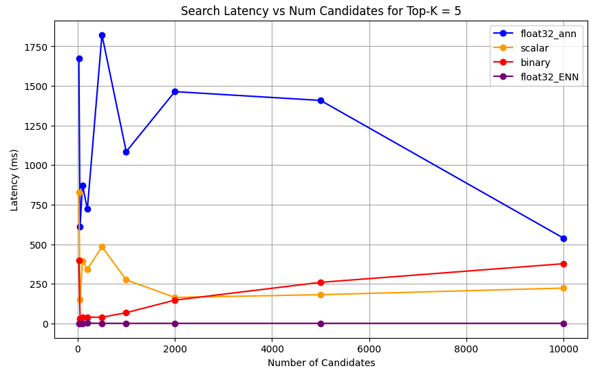
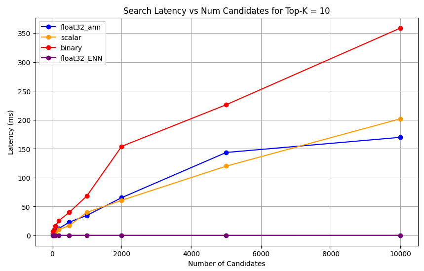
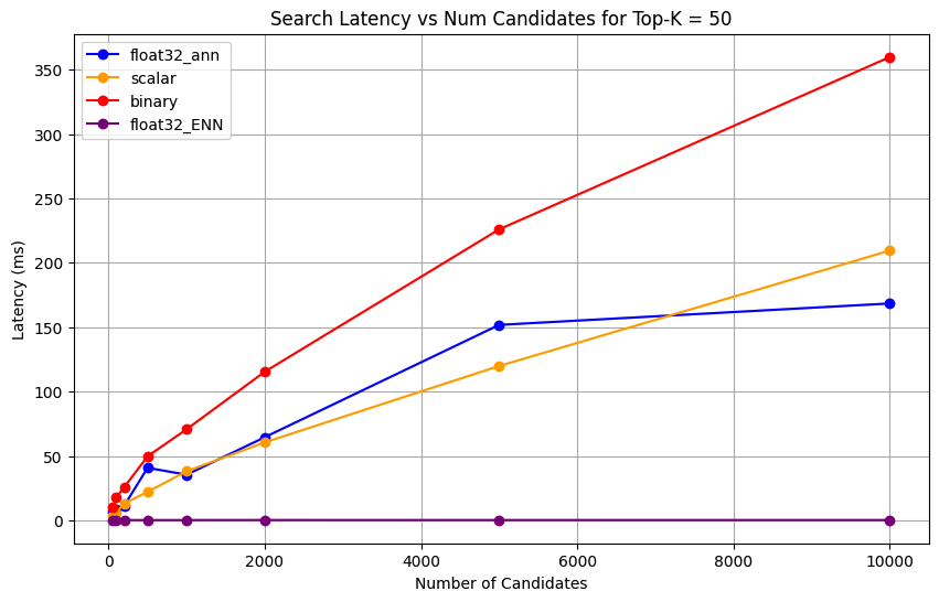
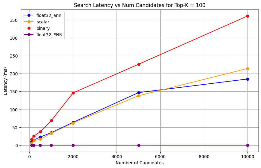
1 # Run the measurements 2 user_query = "How do I increase my productivity for maximum output" 3 top_k_values = [5, 10, 50, 100] 4 num_candidates_values = [25, 50, 100, 200, 500, 1000, 2000, 5000, 10000] 5 6 latency_results = [] 7 8 for vector_search_index in vector_search_indices: 9 latency_results.append( 10 measure_latency_with_varying_topk( 11 user_query, 12 wiki_data_collection, 13 vector_search_index_name=vector_search_index, 14 use_full_precision=False, 15 top_k_values=top_k_values, 16 num_candidates_values=num_candidates_values, 17 ) 18 ) 19 20 # Conduct vector search operation using full precision 21 latency_results.append( 22 measure_latency_with_varying_topk( 23 user_query, 24 wiki_data_collection, 25 vector_search_index_name="vector_index_scalar_quantized", 26 use_full_precision=True, 27 top_k_values=top_k_values, 28 num_candidates_values=num_candidates_values, 29 ) 30 ) The latency measurements reveal a clear performance hierarchy across precision types, where binary quantization demonstrates the fastest retrieval times, followed by scalar quantization. The full precision float32 ANN operations show significantly higher latencies. The performance gap between quantized and full precision searches become more pronounced as Top-K values increase. The float32 ENN operations are the slowest, but they provide the highest precision results.
さまざまなトップk値に対する検索レイテンシをプロットします。
1 import matplotlib.pyplot as plt 2 3 # Map your precision field to the labels and colors you want in the legend 4 precision_label_map = { 5 "_scalar_": "scalar", 6 "_binary_": "binary", 7 "_float32_ann": "float32_ann", 8 "_float32_ENN": "float32_ENN", 9 } 10 11 precision_color_map = { 12 "_scalar_": "orange", 13 "_binary_": "red", 14 "_float32_ann": "blue", 15 "_float32_ENN": "purple", 16 } 17 18 # Flatten all measurements and find the unique top_k values 19 all_measurements = [m for precision_list in latency_results for m in precision_list] 20 unique_topk = sorted(set(m["top_k"] for m in all_measurements)) 21 22 # For each top_k, create a separate plot 23 for k in unique_topk: 24 plt.figure(figsize=(10, 6)) 25 26 # For each precision type, filter out measurements for the current top_k value 27 for measurements in latency_results: 28 # Filter measurements with top_k equal to the current k 29 filtered = [m for m in measurements if m["top_k"] == k] 30 if not filtered: 31 continue 32 33 # Extract x (num_candidates) and y (latency) values 34 x = [m["num_candidates"] for m in filtered] 35 y = [m["latency_ms"] for m in filtered] 36 37 # Determine the precision, label, and color from the first measurement in this filtered list 38 precision = filtered[0]["precision"] 39 label = precision_label_map.get(precision, precision) 40 color = precision_color_map.get(precision, "blue") 41 42 # Plot the line for this precision type 43 plt.plot(x, y, marker="o", color=color, label=label) 44 45 # Label axes and add title including the top_k value 46 plt.xlabel("Number of Candidates") 47 plt.ylabel("Latency (ms)") 48 plt.title(f"Search Latency vs Num Candidates for Top-K = {k}") 49 50 # Add a legend and grid, then show the plot 51 plt.legend() 52 plt.grid(True) 53 plt.show() このコードは次のレイテンシチャートを返します。これは、
top-k(取得される結果の数)が増加するにつれて、バイナリ、スカラー、float32などのさまざまな埋め込み精度タイプでベクトル検索ドキュメントの検索がどのように実行されるかを示しています。
表現キャパシティーとリテンションを測定します。
次のクエリは、 MongoDB ベクトル検索 が基礎データセットから関連ドキュメントをどの程度効果的に検索するかを測定します。これは、フィールド 真実の関連ドキュメントの総数 (Found/ Total) に対する関連ドキュメントの総数に対する比率として計算されます。例、クエリにフィールド 真実の関連ドキュメントが 5 あり、 MongoDB ベクトル検索 がそれらのドキュメントの 4 を見つけた場合、呼び出しは 0.8 になりますまたは 80%。
ベクトル検索操作の表現能力と保持力を測定する関数を定義します。この関数は次の処理を行います。
フル精度の float32 ベクトルと 厳密最近傍探索 を使用してベースライン検索を作成します。
量子化ベクトルと近似最近傍探索を使用して量子化検索を作成します。
量子化検索の保持率をベースライン検索と比較して計算します。
量子化検索のために、保持は合理的な範囲内で維持されなければなりません。表現能力が低い場合、ベクトル検索操作がクエリのセマンティックな意味を捉えられず、結果が正確でない可能性があります。これは、量子化が効果的ではなく、使用された初期の埋め込みモデルが量子化プロセスに適していないことを示しています。量子化に対応した埋め込みモデルの利用をお勧めします。これは、訓練プロセス中に、量子化後もセマンティックな特性を維持するようにモデルが特別に最適化されていることを意味します。
1 def measure_representational_capacity_retention_against_float_enn( 2 ground_truth_collection, 3 collection, 4 quantized_index_name, # This is used for both the quantized search and (with use_full_precision=True) for the baseline. 5 top_k_values, # List/array of top-k values to test. 6 num_candidates_values, # List/array of num_candidates values to test. 7 num_queries_to_test=1, 8 ): 9 retention_results = {"per_query_retention": {}} 10 overall_retention = {} # overall_retention[top_k][num_candidates] = [list of retention values] 11 12 # Initialize overall retention structure 13 for top_k in top_k_values: 14 overall_retention[top_k] = {} 15 for num_candidates in num_candidates_values: 16 if num_candidates < top_k: 17 continue 18 overall_retention[top_k][num_candidates] = [] 19 20 # Extract and store the precision name from the quantized index name. 21 precision_name = quantized_index_name.split("vector_index")[1] 22 precision_name = precision_name.replace("quantized", "").capitalize() 23 retention_results["precision_name"] = precision_name 24 retention_results["top_k_values"] = top_k_values 25 retention_results["num_candidates_values"] = num_candidates_values 26 27 # Load ground truth annotations 28 ground_truth_annotations = list( 29 ground_truth_collection.find().limit(num_queries_to_test) 30 ) 31 print(f"Loaded {len(ground_truth_annotations)} ground truth annotations") 32 33 # Process each ground truth annotation 34 for annotation in ground_truth_annotations: 35 # Use the ground truth wiki_id from the annotation. 36 ground_truth_wiki_id = annotation["wiki_id"] 37 38 # Process only queries that are questions. 39 for query_type, queries in annotation["queries"].items(): 40 if query_type.lower() not in ["question", "questions"]: 41 continue 42 43 for query in queries: 44 # Prepare nested dict for this query 45 if query not in retention_results["per_query_retention"]: 46 retention_results["per_query_retention"][query] = {} 47 48 # For each valid combination of top_k and num_candidates 49 for top_k in top_k_values: 50 if top_k not in retention_results["per_query_retention"][query]: 51 retention_results["per_query_retention"][query][top_k] = {} 52 for num_candidates in num_candidates_values: 53 if num_candidates < top_k: 54 continue 55 56 # Baseline search: full precision using ENN (Float32) 57 baseline_result = custom_vector_search( 58 user_query=query, 59 collection=collection, 60 embedding_path="embedding", 61 vector_search_index_name=quantized_index_name, 62 top_k=top_k, 63 num_candidates=num_candidates, 64 use_full_precision=True, 65 ) 66 baseline_ids = { 67 res["wiki_id"] for res in baseline_result["results"] 68 } 69 70 # Quantized search: 71 quantized_result = custom_vector_search( 72 user_query=query, 73 collection=collection, 74 embedding_path="embedding", 75 vector_search_index_name=quantized_index_name, 76 top_k=top_k, 77 num_candidates=num_candidates, 78 use_full_precision=False, 79 ) 80 quantized_ids = { 81 res["wiki_id"] for res in quantized_result["results"] 82 } 83 84 # Compute retention for this combination 85 if baseline_ids: 86 retention = len( 87 baseline_ids.intersection(quantized_ids) 88 ) / len(baseline_ids) 89 else: 90 retention = 0 91 92 # Store the results per query 93 retention_results["per_query_retention"][query].setdefault( 94 top_k, {} 95 )[num_candidates] = { 96 "ground_truth_wiki_id": ground_truth_wiki_id, 97 "baseline_ids": sorted(baseline_ids), 98 "quantized_ids": sorted(quantized_ids), 99 "retention": retention, 100 } 101 overall_retention[top_k][num_candidates].append(retention) 102 103 print( 104 f"Query: '{query}' | top_k: {top_k}, num_candidates: {num_candidates}" 105 ) 106 print(f" Ground Truth wiki_id: {ground_truth_wiki_id}") 107 print(f" Baseline IDs (Float32): {sorted(baseline_ids)}") 108 print( 109 f" Quantized IDs: {precision_name}: {sorted(quantized_ids)}" 110 ) 111 print(f" Retention: {retention:.4f}\n") 112 113 # Compute overall average retention per combination 114 avg_overall_retention = {} 115 for top_k, cand_dict in overall_retention.items(): 116 avg_overall_retention[top_k] = {} 117 for num_candidates, retentions in cand_dict.items(): 118 if retentions: 119 avg = sum(retentions) / len(retentions) 120 else: 121 avg = 0 122 avg_overall_retention[top_k][num_candidates] = avg 123 print( 124 f"Overall Average Retention for top_k {top_k}, num_candidates {num_candidates}: {avg:.4f}" 125 ) 126 127 retention_results["average_retention"] = avg_overall_retention 128 return retention_results MongoDB ベクトル検索インデックスのパフォーマンスを評価して比較します。
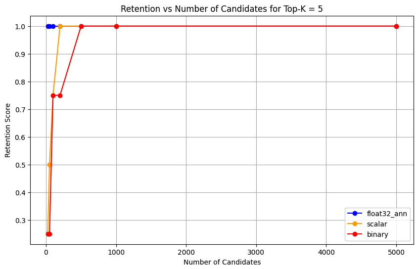
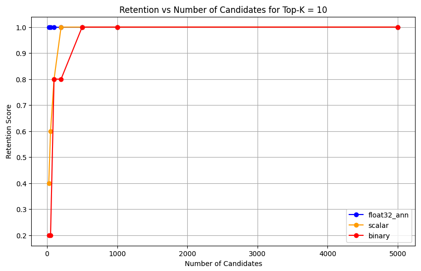
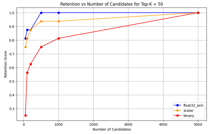
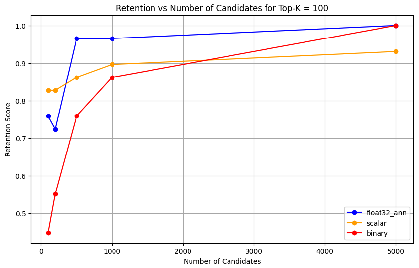
1 # Access the database 2 DB_NAME = "testing_datasets" 3 db = mongo_client[DB_NAME] 4 5 # Access collections 6 wiki_data_collection = db["wikipedia-22-12-en"] 7 ground_truth_collection = db["wikipedia-22-12-en-annotation"] 8 9 overall_recall_results = [] 10 top_k_values = [5, 10, 50, 100] 11 num_candidates_values = [25, 50, 100, 200, 500, 1000, 5000] 12 num_queries_to_test = 1 13 14 for vector_search_index in vector_search_indices: 15 overall_recall_results.append( 16 measure_representational_capacity_retention_against_float_enn( 17 ground_truth_collection=ground_truth_collection, 18 collection=wiki_data_collection, 19 quantized_index_name=vector_search_index, 20 top_k_values=top_k_values, 21 num_candidates_values=num_candidates_values, 22 num_queries_to_test=num_queries_to_test, 23 ) 24 ) 出力には、グラウンド トゥルース データセット内の各クエリの保持結果が表示されます。保持は 0 から 1 までの小数で表されます。1.0 はグラウンド トゥルース ID が保持されることを意味し、0.25 はグラウンド トゥルース ID の 25% のみが保持されることを意味します。
さまざまな精度タイプの保持機能をプロットしてください。
1 import matplotlib.pyplot as plt 2 3 # Define colors and labels for each precision type 4 precision_colors = {"_scalar_": "orange", "_binary_": "red", "_float32_": "green"} 5 6 if overall_recall_results: 7 # Determine unique top_k values from the first result's average_retention keys 8 unique_topk = sorted(list(overall_recall_results[0]["average_retention"].keys())) 9 10 for k in unique_topk: 11 plt.figure(figsize=(10, 6)) 12 # For each precision type, plot retention vs. number of candidates at this top_k 13 for result in overall_recall_results: 14 precision_name = result.get("precision_name", "unknown") 15 color = precision_colors.get(precision_name, "blue") 16 # Get candidate values from the average_retention dictionary for top_k k 17 candidate_values = sorted(result["average_retention"][k].keys()) 18 retention_values = [ 19 result["average_retention"][k][nc] for nc in candidate_values 20 ] 21 22 plt.plot( 23 candidate_values, 24 retention_values, 25 marker="o", 26 label=precision_name.strip("_"), 27 color=color, 28 ) 29 30 plt.xlabel("Number of Candidates") 31 plt.ylabel("Retention Score") 32 plt.title(f"Retention vs Number of Candidates for Top-K = {k}") 33 plt.legend() 34 plt.grid(True) 35 plt.show() 36 37 # Print detailed average retention results 38 print("\nDetailed Average Retention Results:") 39 for result in overall_recall_results: 40 precision_name = result.get("precision_name", "unknown") 41 print(f"\n{precision_name} Embedding:") 42 for k in sorted(result["average_retention"].keys()): 43 print(f"\nTop-K: {k}") 44 for nc in sorted(result["average_retention"][k].keys()): 45 ret = result["average_retention"][k][nc] 46 print(f" NumCandidates: {nc}, Retention: {ret:.4f}") このコードは、次のリテンション チャートを返します。
float32_ann、scalar、binaryの埋め込みに対して、コードは以下のような詳細な平均保持結果も返します。Detailed Average Retention Results: _float32_ann Embedding: Top-K: 5 NumCandidates: 25, Retention: 1.0000 NumCandidates: 50, Retention: 1.0000 NumCandidates: 100, Retention: 1.0000 NumCandidates: 200, Retention: 1.0000 NumCandidates: 500, Retention: 1.0000 NumCandidates: 1000, Retention: 1.0000 NumCandidates: 5000, Retention: 1.0000 Top-K: 10 NumCandidates: 25, Retention: 1.0000 NumCandidates: 50, Retention: 1.0000 NumCandidates: 100, Retention: 1.0000 NumCandidates: 200, Retention: 1.0000 NumCandidates: 500, Retention: 1.0000 NumCandidates: 1000, Retention: 1.0000 NumCandidates: 5000, Retention: 1.0000 Top-K: 50 NumCandidates: 50, Retention: 0.8125 NumCandidates: 100, Retention: 0.8750 NumCandidates: 200, Retention: 0.8750 NumCandidates: 500, Retention: 1.0000 NumCandidates: 1000, Retention: 1.0000 NumCandidates: 5000, Retention: 1.0000 Top-K: 100 NumCandidates: 100, Retention: 0.7586 NumCandidates: 200, Retention: 0.7241 NumCandidates: 500, Retention: 0.9655 NumCandidates: 1000, Retention: 0.9655 NumCandidates: 5000, Retention: 1.0000 _scalar_ Embedding: Top-K: 5 NumCandidates: 25, Retention: 0.2500 NumCandidates: 50, Retention: 0.5000 NumCandidates: 100, Retention: 0.7500 NumCandidates: 200, Retention: 1.0000 NumCandidates: 500, Retention: 1.0000 NumCandidates: 1000, Retention: 1.0000 NumCandidates: 5000, Retention: 1.0000 Top-K: 10 NumCandidates: 25, Retention: 0.4000 NumCandidates: 50, Retention: 0.6000 NumCandidates: 100, Retention: 0.8000 NumCandidates: 200, Retention: 1.0000 NumCandidates: 500, Retention: 1.0000 NumCandidates: 1000, Retention: 1.0000 NumCandidates: 5000, Retention: 1.0000 Top-K: 50 NumCandidates: 50, Retention: 0.7500 NumCandidates: 100, Retention: 0.8125 NumCandidates: 200, Retention: 0.8750 NumCandidates: 500, Retention: 0.9375 NumCandidates: 1000, Retention: 0.9375 NumCandidates: 5000, Retention: 1.0000 Top-K: 100 NumCandidates: 100, Retention: 0.8276 NumCandidates: 200, Retention: 0.8276 NumCandidates: 500, Retention: 0.8621 NumCandidates: 1000, Retention: 0.8966 NumCandidates: 5000, Retention: 0.9310 _binary_ Embedding: Top-K: 5 NumCandidates: 25, Retention: 0.2500 NumCandidates: 50, Retention: 0.2500 NumCandidates: 100, Retention: 0.7500 NumCandidates: 200, Retention: 0.7500 NumCandidates: 500, Retention: 1.0000 NumCandidates: 1000, Retention: 1.0000 NumCandidates: 5000, Retention: 1.0000 Top-K: 10 NumCandidates: 25, Retention: 0.2000 NumCandidates: 50, Retention: 0.2000 NumCandidates: 100, Retention: 0.8000 NumCandidates: 200, Retention: 0.8000 NumCandidates: 500, Retention: 1.0000 NumCandidates: 1000, Retention: 1.0000 NumCandidates: 5000, Retention: 1.0000 Top-K: 50 NumCandidates: 50, Retention: 0.2500 NumCandidates: 100, Retention: 0.5625 NumCandidates: 200, Retention: 0.6250 NumCandidates: 500, Retention: 0.7500 NumCandidates: 1000, Retention: 0.8125 NumCandidates: 5000, Retention: 1.0000 Top-K: 100 NumCandidates: 100, Retention: 0.4483 NumCandidates: 200, Retention: 0.5517 NumCandidates: 500, Retention: 0.7586 NumCandidates: 1000, Retention: 0.8621 NumCandidates: 5000, Retention: 1.0000 リコール結果は、3 つの埋め込みタイプ間で異なるパフォーマンス パターンを示しています。
スカラー量子化は着実な改善を示し、より高い K 値で強力な検索精度を示しています。2 進量子化は、最初は低いものの、Top-K 50 と Top-K 100 で改善し、計算効率とリコール性能のトレードオフを示唆しています。float32 の埋め込みは、最も強力な初期パフォーマンスを示し、Top-K 50 および Top-K 100 でスカラー量子化と同じ最大リコールに達します。
これは、float32 が低い Top-K 値でより高い再現率を提供する一方で、スカラー量子化は計算効率を向上させつつ、高い Top-K 値でも同等のパフォーマンスを達成できることを示唆しています。2 進量子化は、リコールの上限が低いにもかかわらず、メモリおよび計算の制約が最大限のリコール精度の必要性を上回るシナリオでは依然として価値があるかもしれません。