AI 애플리케이션은 종종 컴퓨팅, 데이터, 비용 측면에서 소규모로 시작할 수 있습니다. 프로덕션 애플리케이션이 사용자 참여 증가로 인해 확장됨에 따라, 대규모 데이터의 저장 및 검색과 관련된 비용과 같은 주요 요소가 중요한 최적화 기회로 부상합니다. 이러한 문제들은 아래에 집중함으로써 해결할 수 있습니다.
효율적인 벡터 검색 알고리즘
자동화된 양자화 프로세스
최적화된 임베딩 전략
검색 증강 생성(RAG)과 에이전트 기반 시스템은 모두 벡터 데이터(이미지, 비디오, 텍스트와 같은 데이터 객체의 수치적 표현)를 사용하여 의미적 유사성 검색을 수행합니다. RAG 또는 에이전트 기반 워크플로우를 사용하는 시스템은 빠른 응답 시간을 유지하고 검색 지연 시간을 최소화하며, 인프라 비용을 관리하기 위해 대규모 고차원 데이터 세트를 효율적으로 처리해야 합니다.
튜토리얼 소개
이 튜토리얼은 대규모로 고급 AI 워크로드를 설계, 배포 및 관리하는 데 필요한 기술을 제공하여 최적의 성능과 비용 효율성을 보장합니다.
구체적으로 이 튜토리얼에서 배우게 될 내용은 다음과 같습니다.
Voyage AI의
voyage-3-large를 사용하여 임베딩을 생성하세요. 이 모델은 범용적이며 다국어 지원, 양자화 인지도 갖춘 임베딩 모델로, 생성한 임베딩을 MongoDB 데이터베이스에 삽입할 수 있습니다.임베딩을 자동으로 양자화하여 낮은 정밀도의 데이터 유형으로 변환함으로써 메모리 사용량과 쿼리 지연 시간을 최적화합니다.
float32, int8 및 바이너리 임베딩을 비교하는 쿼리를 실행하여 데이터 유형의 정밀도, 효율성 및 검색 정확도를 평가합니다.
양자화된 임베딩의 재현율(또는 보존율)을 측정합니다. 이는 양자화된 근사 최근접 이웃 검색이 고정밀 등가 최근접 이웃 검색과 동일한 문서를 얼마나 효과적으로 조회하는지 평가합니다.
참고
이진 양자화는 리소스 소비를 줄여야 하는 시나리오에 최적이지만 정확도 손실을 보완하기 위해 재스코어링이 필요할 수 있습니다.
스칼라 양자화는 성능과 정밀성의 균형이 필요한 대부분의 사용 사례에 적합한 실용적인 중간 솔루션을 제공합니다.
Float32는 최대의 정밀도를 보장하지만, 성능 및 메모리 오버헤드가 가장 크기 때문에 대규모나 지연에 민감한 시스템에는 적합하지 않습니다.
전제 조건
이 튜토리얼을 완료하려면 다음 조건을 충족해야 합니다.
절차
필요한 라이브러리를 가져오고 환경 변수를 설정합니다.
확장자가
.ipynb인 파일 을 저장하여 대화형 Python 노트북을 만듭니다.라이브러리를 설치합니다.
이 튜토리얼에서는 다음 라이브러리를 반드시 가져와야 합니다.
pymongo
MongoDB Python 운전자 사용하여 클러스터 에 연결하고, 인덱스를 생성하고, 쿼리를 실행 .
voyageai
Voyage AI Python 클라이언트를 사용해 데이터 임베딩을 생성합니다.
pandas
데이터를 로드하고 벡터검색 위해 준비하는 데이터 조작 및 분석 도구입니다.
데이터 세트
Hugging Face 라이브러리는 미리 준비된 데이터 세트에 액세스할 수 있게 해줍니다.
matplotlib
라이브러리를 플로팅 및 시각화 하여 데이터를 시각화합니다.
라이브러리를 설치하려면 다음을 실행합니다.
pip install --quiet -U pymongo voyageai pandas datasets matplotlib 환경 변수를 안전하게 가져오고 설정합니다.
다음
set_env_securely헬퍼 함수는 환경 변수를 안전하게 가져오고 설정합니다. 다음 코드를 복사하여 붙여넣은 후 실행 하고 메시지가 표시되면 Voyage AI API 키 및 클러스터 연결 문자열 과 같은 시크릿 값을 설정하다 .1 import getpass 2 import os 3 import voyageai 4 5 # Function to securely get and set environment variables 6 def set_env_securely(var_name, prompt): 7 value = getpass.getpass(prompt) 8 os.environ[var_name] = value 9 10 # Environment Variables 11 set_env_securely("VOYAGE_API_KEY", "Enter your Voyage API Key: ") 12 set_env_securely("MONGO_URI", "Enter your MongoDB URI: ") 13 MONGO_URI = os.environ.get("MONGO_URI") 14 if not MONGO_URI: 15 raise ValueError("MONGO_URI not set in environment variables.") 16 17 # Voyage Client 18 voyage_client = voyageai.Client()
클러스터 로 데이터를 수집합니다.
이 단계에서는 다음 데이터셋에서 최대 250000개의 문서를 불러옵니다.
wikipedia-22-12-en-voyage-embed 데이터 세트에는 Voyage AI의 voyage-3-large 모델에서 미리 생성된 1024차원 float32 임베딩이 있는 Wikipedia 문서 조각이 포함되어 있습니다. 이는 메타데이터 포함된 프라이머리 문서 컬렉션 입니다. 이 데이터 세트는 시맨틱 검색 에서 벡터 양자화 효과를 테스트하기 위한 다양한 벡터 코퍼스 역할을 합니다. 이 데이터 세트의 각 문서 에는 다음 필드가 포함되어 있습니다.
| 문서의 ObjectId( |
| 문서의 고유 식별자입니다. |
| 문서의 제목입니다. |
| 문서의 텍스트입니다. |
| 문서의 URL입니다. |
| 문서의 Wikipedia ID입니다. |
| 문서의 조회수입니다. |
| 문서 내 단락 ID입니다. |
| 문서에 포함된 언어의 수입니다. |
| 문서에 대한 1024차원 벡터 임베딩입니다. |
wikipedia-22-12-en-annotation 데이터 세트에는 리콜 측정 함수에 대한 주석이 달린 참조 데이터가 포함되어 있습니다. 이 데이터는 정확도 유효성 검사 위한 벤치마크 데이터 세트로 사용되며, 양자화가 검색 품질에 영향 평가합니다. 이 데이터 세트의 각 문서 에는 벡터 검색 의 성능을 평가하는 데 사용되는 실측값인 다음 필드가 포함되어 있습니다.
| 문서의 ObjectId( |
| 문서의 고유 식별자입니다. |
| 문서의 Wikipedia ID입니다. |
| 문서의 핵심 구문, 질문, 부분 정보 및 문장을 포함하는 쿼리입니다. |
| 문서의 벡터 검색 성능을 평가하는 데 사용되는 주요 구문의 배열입니다. |
| 문서의 벡터 검색 성능 평가에 사용되는 부분 정보 배열입니다. |
| 문서의 벡터 검색 성능을 평가하기 위해 사용되는 질문 배열입니다. |
| 문서의 벡터 검색 성능을 평가하는 데 사용되는 문장 배열입니다. |
클러스터에 데이터를 로드할 함수를 정의하세요.
다음 코드를 복사 및 붙여넣기하여 노트북에서 실행하세요. 샘플 코드는 다음 함수를 정의합니다.
generate_bson_vector로 데이터셋의 임베딩을 BSON 이진 벡터로 변환하여 벡터를 효율적으로 저장하고 처리할 수 있습니다.get_mongo_client클러스터 연결 문자열 가져옵니다.insert_dataframe_into_collection클러스터 로 데이터를 수집합니다.
1 import pandas as pd 2 from datasets import load_dataset 3 from bson.binary import Binary, BinaryVectorDtype 4 import pymongo 5 6 # Connect to Cluster 7 def get_mongo_client(uri): 8 """Connect to MongoDB and confirm the connection.""" 9 client = pymongo.MongoClient(uri) 10 if client.admin.command("ping").get("ok") == 1.0: 11 print("Connected to MongoDB successfully.") 12 return client 13 print("Failed to connect to MongoDB.") 14 return None 15 16 # Generate BSON Vector 17 def generate_bson_vector(array, data_type): 18 """Convert an array to BSON vector format.""" 19 array = [float(val) for val in eval(array)] 20 return Binary.from_vector(array, BinaryVectorDtype(data_type)) 21 22 # Load Datasets 23 def load_and_prepare_data(dataset_name, amount): 24 """Load and prepare streaming datasets for DataFrame.""" 25 data = load_dataset(dataset_name, streaming=True, split="train").take(amount) 26 return pd.DataFrame(data) 27 28 # Insert datasets into MongoDB Collection 29 def insert_dataframe_into_collection(df, collection): 30 """Insert Dataset records into MongoDB collection.""" 31 collection.insert_many(df.to_dict("records")) 32 print(f"Inserted {len(df)} records into '{collection.name}' collection.") 클러스터에 데이터를 로드합니다.
노트북에서 다음 코드를 복사하여 붙여넣고 실행 클러스터 에 데이터 세트를 로드합니다. 이 코드는 다음 작업을 수행합니다.
데이터셋을 가져옵니다.
임베딩을 BSON 형식으로 변환합니다.
클러스터 에 컬렉션을 생성하고 데이터를 삽입합니다.
1 import pandas as pd 2 from bson.binary import Binary, BinaryVectorDtype 3 from pymongo.errors import CollectionInvalid 4 5 wikipedia_data_df = load_and_prepare_data("MongoDB/wikipedia-22-12-en-voyage-embed", amount=250000) 6 wikipedia_annotation_data_df = load_and_prepare_data("MongoDB/wikipedia-22-12-en-annotation", amount=250000) 7 wikipedia_annotation_data_df.drop(columns=["_id"], inplace=True) 8 9 # Convert embeddings to BSON format 10 wikipedia_data_df["embedding"] = wikipedia_data_df["embedding"].apply( 11 lambda x: generate_bson_vector(x, BinaryVectorDtype.FLOAT32) 12 ) 13 14 # MongoDB Setup 15 mongo_client = get_mongo_client(MONGO_URI) 16 DB_NAME = "testing_datasets" 17 db = mongo_client[DB_NAME] 18 19 collections = { 20 "wikipedia-22-12-en": wikipedia_data_df, 21 "wikipedia-22-12-en-annotation": wikipedia_annotation_data_df, 22 } 23 24 # Create Collections and Insert Data 25 for collection_name, df in collections.items(): 26 if collection_name not in db.list_collection_names(): 27 try: 28 db.create_collection(collection_name) 29 print(f"Collection '{collection_name}' created successfully.") 30 except CollectionInvalid: 31 print(f"Error creating collection '{collection_name}'.") 32 else: 33 print(f"Collection '{collection_name}' already exists.") 34 35 # Clear collection and insert fresh data 36 collection = db[collection_name] 37 collection.delete_many({}) 38 insert_dataframe_into_collection(df, collection) Connected to MongoDB successfully. Collection 'wikipedia-22-12-en' created successfully. Inserted 250000 records into 'wikipedia-22-12-en' collection. Collection 'wikipedia-22-12-en-annotation' created successfully. Inserted 87200 records into 'wikipedia-22-12-en-annotation' collection. 참고 사항: 임베딩을 BSON 벡터로 변환하고 데이터 세트를 클러스터로 수집하는 데 시간이 걸릴 수 있습니다.
클러스터에 로그인하고 데이터 탐색기에서 컬렉션을 시각적으로 검사하여 데이터 세트가 성공적으로 로드되었는지 확인합니다.
컬렉션 에 MongoDB Vector Search 인덱스를 생성합니다.
embedding 필드에 다음 세 가지 인덱스를 생성합니다.
스칼라 양자화 인덱스 | 스칼라 양자화 방법을 사용하여 임베딩을 양자화합니다. |
이진 양자화 인덱스 | 이진 양자화 방법을 사용해 임베딩을 양자화합니다. |
Float32 ANN Index | float32 근사 최근접 이웃 메서드를 사용하여 임베딩을 양자화합니다. |
MongoDB Vector Search 인덱스 생성하는 함수를 정의합니다.
다음 코드를 복사하여 노트북에 붙여넣고 실행합니다.
1 import time 2 from pymongo.operations import SearchIndexModel 3 4 def setup_vector_search_index(collection, index_definition, index_name="vector_index"): 5 new_vector_search_index_model = SearchIndexModel( 6 definition=index_definition, name=index_name, type="vectorSearch" 7 ) 8 9 # Create the new index 10 try: 11 result = collection.create_search_index(model=new_vector_search_index_model) 12 print(f"Creating index '{index_name}'...") 13 14 # Wait for initial sync to complete 15 print("Polling to check if the index is ready. This may take a couple of minutes.") 16 predicate=None 17 if predicate is None: 18 predicate = lambda index: index.get("queryable") is True 19 while True: 20 indices = list(collection.list_search_indexes(result)) 21 if len(indices) and predicate(indices[0]): 22 break 23 time.sleep(5) 24 print(f"Index '{index_name}' is ready for querying.") 25 return result 26 27 except Exception as e: 28 print(f"Error creating new vector search index '{index_name}': {e!s}") 29 return None 인덱스를 정의합니다.
다음 인덱스 구성은 서로 다른 양자화 전략을 구현합니다.
vector_index_definition_scalar_quantized이 구성은 스칼라 양자화(int8)를 사용합니다. 이는 다음과 같습니다.
각 벡터 차원을 32비트 부동소수점에서 8비트 정수로 변환
정밀도와 메모리 효율성 간의 좋은 균형을 유지
메모리 최적화가 필요한 대부분의 프로덕션 사용 사례에 적합
vector_index_definition_binary_quantized이 구성은 이진 양자화(int1)를 사용합니다. 이는 다음과 같습니다.
각 벡터 차원을 하나의 비트로 줄입니다
최대 메모리 효율성을 제공합니다.
메모리 제약이 매우 중요한 대규모 배포에 이상적
자동 양자화는 이러한 인덱스가 생성될 때 투명하게 발생하며, MongoDB Vector Search는 인덱스 생성 및 검색 작업 중에 float32 에서 지정된 양자화된 형식으로의 변환을 처리합니다.
vector_index_definition_float32_ann인덱스 구성은1024차원의 전체 정밀도 벡터를cosine유사도 함수를 사용해 인덱싱합니다.1 # Scalar Quantization 2 vector_index_definition_scalar_quantized = { 3 "fields": [ 4 { 5 "type": "vector", 6 "path": "embedding", 7 "quantization": "scalar", 8 "numDimensions": 1024, 9 "similarity": "cosine", 10 } 11 ] 12 } 13 # Binary Quantization 14 vector_index_definition_binary_quantized = { 15 "fields": [ 16 { 17 "type": "vector", 18 "path": "embedding", 19 "quantization": "binary", 20 "numDimensions": 1024, 21 "similarity": "cosine", 22 } 23 ] 24 } 25 # Float32 Embeddings 26 vector_index_definition_float32_ann = { 27 "fields": [ 28 { 29 "type": "vector", 30 "path": "embedding", 31 "numDimensions": 1024, 32 "similarity": "cosine", 33 } 34 ] 35 } setup_vector_search_index함수를 사용하여 스칼라, 이진 그리고 부동 소수점32 인덱스를 생성합니다.인덱스를 위한 컬렉션 이름과 인덱스 이름을 설정합니다.
wiki_data_collection = db["wikipedia-22-12-en"] wiki_annotation_data_collection = db["wikipedia-22-12-en-annotation"] vector_search_scalar_quantized_index_name = "vector_index_scalar_quantized" vector_search_binary_quantized_index_name = "vector_index_binary_quantized" vector_search_float32_ann_index_name = "vector_index_float32_ann" MongoDB Vector Search 인덱스를 생성합니다.
1 setup_vector_search_index( 2 wiki_data_collection, 3 vector_index_definition_scalar_quantized, 4 vector_search_scalar_quantized_index_name, 5 ) 6 setup_vector_search_index( 7 wiki_data_collection, 8 vector_index_definition_binary_quantized, 9 vector_search_binary_quantized_index_name, 10 ) 11 setup_vector_search_index( 12 wiki_data_collection, 13 vector_index_definition_float32_ann, 14 vector_search_float32_ann_index_name, 15 ) Creating index 'vector_index_scalar_quantized'... Polling to check if the index is ready. This may take a couple of minutes. Index 'vector_index_scalar_quantized' is ready for querying. Creating index 'vector_index_binary_quantized'... Polling to check if the index is ready. This may take a couple of minutes. Index 'vector_index_binary_quantized' is ready for querying. Creating index 'vector_index_float32_ann'... Polling to check if the index is ready. This may take a couple of minutes. Index 'vector_index_float32_ann' is ready for querying. vector_index_float32_ann' 중요: 작업을 완료하는 데 몇 분 정도 걸릴 수 있습니다. 인덱스를 쿼리에서 사용하려면 Ready 상태여야 합니다.
클러스터 에 로그인하고 Atlas Search의 인덱스를 시각적으로 검사하여 인덱스 생성이 성공했는지 확인합니다.
MongoDB Vector Search 인덱스를 사용하여 임베딩을 생성하고 컬렉션 쿼리 함수를 정의합니다.
이 코드는 다음 함수를 정의합니다.
get_embedding()함수는 Voyage AI의voyage-3-large임베딩 모델을 사용하여 주어진 텍스트에 대한 1024차원 임베딩을 생성합니다.custom_vector_search함수는 다음 입력 매개변수를 받아 벡터 검색 작업의 결과를 반환합니다.user_query임베딩을 생성하기 위한 쿼리 텍스트 문자열입니다.
collection검색할 MongoDB 컬렉션
embedding_path임베딩을 포함하는 컬렉션의 필드입니다.
vector_search_index_name쿼리에 사용할 인덱스 이름입니다.
top_k결과에서 반환할 상위 문서의 수입니다.
num_candidates고려할 후보 수입니다.
use_full_precisionFalse일 때 근사 최근접 이웃 검색을,True일 때 등가 최근접 이웃 검색을 수행할지 결정하는 플래그입니다.use_full_precision값은 근사 최근접 이웃 검색에서는 기본적으로False로 설정됩니다.use_full_precision값을True로 설정하여 등가 최근접 이웃 검색을 수행합니다.구체적으로, 이 함수는 다음 작업을 수행합니다.
쿼리 텍스트에 대한 임베딩을 생성합니다.
$vectorSearch단계를 구성합니다.검색 유형을 구성합니다.
반환할 필드를 컬렉션에서 지정합니다
성능 통계를 수집한 후 파이프라인을 실행합니다.
결과를 반환합니다.
1 def get_embedding(text, task_prefix="document"): 2 """Fetch embedding for a given text using Voyage AI.""" 3 if not text.strip(): 4 print("Empty text provided for embedding.") 5 return [] 6 result = voyage_client.embed([text], model="voyage-3-large", input_type=task_prefix) 7 return result.embeddings[0] 8 9 def custom_vector_search( 10 user_query, 11 collection, 12 embedding_path, 13 vector_search_index_name="vector_index", 14 top_k=5, 15 num_candidates=25, 16 use_full_precision=False, 17 ): 18 19 # Generate embedding for the user query 20 query_embedding = get_embedding(user_query, task_prefix="query") 21 22 if query_embedding is None: 23 return "Invalid query or embedding generation failed." 24 25 # Define the vector search stage 26 vector_search_stage = { 27 "$vectorSearch": { 28 "index": vector_search_index_name, 29 "queryVector": query_embedding, 30 "path": embedding_path, 31 "limit": top_k, 32 } 33 } 34 35 # Add numCandidates only for approximate search 36 if not use_full_precision: 37 vector_search_stage["$vectorSearch"]["numCandidates"] = num_candidates 38 else: 39 # Set exact to true for exact search using full precision float32 vectors and running exact search 40 vector_search_stage["$vectorSearch"]["exact"] = True 41 42 project_stage = { 43 "$project": { 44 "_id": 0, 45 "title": 1, 46 "text": 1, 47 "wiki_id": 1, 48 "url": 1, 49 "score": { 50 "$meta": "vectorSearchScore" 51 }, 52 } 53 } 54 55 # Define the aggregate pipeline with the vector search stage and additional stages 56 pipeline = [vector_search_stage, project_stage] 57 58 # Execute the explain command 59 explain_result = collection.database.command( 60 "explain", 61 {"aggregate": collection.name, "pipeline": pipeline, "cursor": {}}, 62 verbosity="executionStats", 63 ) 64 65 # Extract the execution time 66 vector_search_explain = explain_result["stages"][0]["$vectorSearch"] 67 execution_time_ms = vector_search_explain["explain"]["query"]["stats"]["context"][ 68 "millisElapsed" 69 ] 70 71 # Execute the actual query 72 results = list(collection.aggregate(pipeline)) 73 74 return {"results": results, "execution_time_ms": execution_time_ms}
MongoDB Vector Search 쿼리 실행하여 검색 성능을 평가합니다.
다음 쿼리는 다양한 양자화 전략에 걸쳐 벡터 검색을 수행하며 스칼라 양자화, 이진 양자화, 완전 정밀도(float32) 벡터의 성능 지표를 측정합니다. 각 정밀도 수준의 검색 지연 시간도 측정하며, 분석적 비교를 위해 결과 형식을 표준화합니다. 이 쿼리는 "최대 출력을 위해 생산성을 높이려면 어떻게 해야 합니까?"라는 쿼리 문자열에 대해 Voyage AI로 생성된 임베딩을 사용합니다.
쿼리는 정밀도 수준(스칼라, 이진, Float32), 결과 집합 크기(top_k), 밀리초 단위의 쿼리 지연 시간, 조회된 문서 콘텐츠 등 핵심 성능 지표를 results 변수에 저장하여 다양한 양자화 전략 간 검색 성능을 평가할 수 있는 포괄적인 지표를 제공합니다.
1 vector_search_indices = [ 2 vector_search_float32_ann_index_name, 3 vector_search_scalar_quantized_index_name, 4 vector_search_binary_quantized_index_name, 5 ] 6 7 # Random query 8 user_query = "How do I increase my productivity for maximum output" 9 test_top_k = 5 10 test_num_candidates = 25 11 12 # Result is a list of dictionaries with the following headings: precision, top_k, latency_ms, results 13 results = [] 14 15 for vector_search_index in vector_search_indices: 16 # Conduct a vector search operation using scalar quantized 17 vector_search_results = custom_vector_search( 18 user_query, 19 wiki_data_collection, 20 embedding_path="embedding", 21 vector_search_index_name=vector_search_index, 22 top_k=test_top_k, 23 num_candidates=test_num_candidates, 24 use_full_precision=False, 25 ) 26 # Include the precision in the results 27 precision = vector_search_index.split("vector_index")[1] 28 precision = precision.replace("quantized", "").capitalize() 29 30 results.append( 31 { 32 "precision": precision, 33 "top_k": test_top_k, 34 "num_candidates": test_num_candidates, 35 "latency_ms": vector_search_results["execution_time_ms"], 36 "results": vector_search_results["results"][0], # Just taking the first result, modify this to include more results if needed 37 } 38 ) 39 40 # Conduct a vector search operation using full precision 41 precision = "Float32_ENN" 42 vector_search_results = custom_vector_search( 43 user_query, 44 wiki_data_collection, 45 embedding_path="embedding", 46 vector_search_index_name="vector_index_scalar_quantized", 47 top_k=test_top_k, 48 num_candidates=test_num_candidates, 49 use_full_precision=True, 50 ) 51 52 results.append( 53 { 54 "precision": precision, 55 "top_k": test_top_k, 56 "num_candidates": test_num_candidates, 57 "latency_ms": vector_search_results["execution_time_ms"], 58 "results": vector_search_results["results"][0], # Just taking the first result, modify this to include more results if needed 59 } 60 ) 61 62 # Convert the results to a pandas DataFrame with the headings: precision, top_k, latency_ms 63 results_df = pd.DataFrame(results) 64 results_df.columns = ["precision", "top_k", "num_candidates", "latency_ms", "results"] 65 66 # To display the results: 67 results_df.head()
precision top_k num_candidates latency_ms results 0 _float32_ann 5 25 1659.498601 {'title': 'Henry Ford', 'text': 'Ford had deci... 1 _scalar_ 5 25 951.537687 {'title': 'Gross domestic product', 'text': 'F... 2 _binary_ 5 25 344.585193 {'title': 'Great Depression', 'text': 'The fir... 3 Float32_ENN 5 25 0.231693 {'title': 'Great Depression', 'text': 'The fir...
결과의 성능 지표는 정밀도 수준에 따른 지연 시간 차이를 보여줍니다. 이는 양자화가 상당한 성능 향상을 제공하지만, 정밀도와 검색 속도 사이에는 뚜렷한 절충점이 존재함을 보여주며 전체 정밀도 float32 연산은 양자화된 연산에 비해 현저히 더 많은 계산 시간이 필요합니다.
다양한 top-k 및 num_candidates 값을 사용하여 지연 시간 측정합니다.
다음 쿼리는 다양한 정밀도 수준과 검색 규모에서 벡터 검색 성능을 평가하는 체계적인 지연 시간 측정 프레임워크를 소개합니다. top-k 매개변수는 반환할 결과 개수를 결정할 뿐 아니라 MongoDB의 HNSW 그래프 검색에서 numCandidates 매개변수 설정에도 사용됩니다.
값은 MongoDB Vector Search가 ANN 검색 중에 numCandidates 탐색하는 HNSW 그래프 의 노드 수에 영향을 줍니다. 여기서 값이 높을수록 실제 가장 가까운 이웃을 찾을 가능성이 높아지지만 계산 시간이 더 많이 필요합니다.
latency_ms를 사람이 읽을 수 있는 형식으로 변환하는 함수를 정의합니다.1 from datetime import timedelta 2 3 def format_time(ms): 4 """Convert milliseconds to a human-readable format""" 5 delta = timedelta(milliseconds=ms) 6 7 # Extract minutes, seconds, and milliseconds with more precision 8 minutes = delta.seconds // 60 9 seconds = delta.seconds % 60 10 milliseconds = round(ms % 1000, 3) # Keep 3 decimal places for milliseconds 11 12 # Format based on duration 13 if minutes > 0: 14 return f"{minutes}m {seconds}.{milliseconds:03.0f}s" 15 elif seconds > 0: 16 return f"{seconds}.{milliseconds:03.0f}s" 17 else: 18 return f"{milliseconds:.3f}ms" 벡터 검색 쿼리의 지연 시간을 측정할 함수를 정의합니다.
다음 함수는
user_query,collection,vector_search_index_name,use_full_precision값,top_k_values값,num_candidates_values값을 입력받아 벡터 검색의 결과를 반환합니다. 여기서 다음에 유의하세요.top_k와num_candidates값이 증가하면 벡터 검색 연산이 더 많은 문서를 처리하게 되어 검색 시간이 더 오래 걸리므로 지연 시간이 늘어납니다.전체 정밀도 검색(
use_full_precision=True)은 근사 검색(use_full_precision=False)보다 지연 시간이 더 깁니다. 이는 전체 정밀도 검색이 전체 데이터셋을 전체 정밀도 float32 벡터로 탐색하기 때문에 근사 검색보다 시간이 더 오래 걸리기 때문입니다.양자화된 검색은 근사 검색과 양자화된 벡터를 사용하기 때문에 전체 충실도 검색보다 지연 시간이 짧습니다.
1 def measure_latency_with_varying_topk( 2 user_query, 3 collection, 4 vector_search_index_name="vector_index_scalar_quantized", 5 use_full_precision=False, 6 top_k_values=[5, 10, 100], 7 num_candidates_values=[25, 50, 100, 200, 500, 1000, 2000, 5000, 10000], 8 ): 9 results_data = [] 10 11 # Conduct vector search operation for each (top_k, num_candidates) combination 12 for top_k in top_k_values: 13 for num_candidates in num_candidates_values: 14 # Skip scenarios where num_candidates < top_k 15 if num_candidates < top_k: 16 continue 17 18 # Construct the precision name 19 precision_name = vector_search_index_name.split("vector_index")[1] 20 precision_name = precision_name.replace("quantized", "").capitalize() 21 22 # If use_full_precision is true, then the precision name is "_float32_" 23 if use_full_precision: 24 precision_name = "_float32_ENN" 25 26 # Perform the vector search 27 vector_search_results = custom_vector_search( 28 user_query=user_query, 29 collection=collection, 30 embedding_path="embedding", 31 vector_search_index_name=vector_search_index_name, 32 top_k=top_k, 33 num_candidates=num_candidates, 34 use_full_precision=use_full_precision, 35 ) 36 37 # Extract the execution time (latency) 38 latency_ms = vector_search_results["execution_time_ms"] 39 40 # Store results 41 results_data.append( 42 { 43 "precision": precision_name, 44 "top_k": top_k, 45 "num_candidates": num_candidates, 46 "latency_ms": latency_ms, 47 } 48 ) 49 50 return results_data MongoDB Vector Search 쿼리 실행하여 지연 시간 측정합니다.
지연 시간 평가 작업은 모든 양자화 전략에 걸쳐 검색을 실행하고, 다양한 결과 집합 크기를 테스트하며, 표준화된 성능 지표를 수집하고, 비교 분석을 위해 결과를 집계하여 포괄적인 성능 분석을 수행합니다. 이를 통해 다양한 구성 및 검색 부하에서 벡터 검색 동작을 상세히 평가할 수 있습니다.
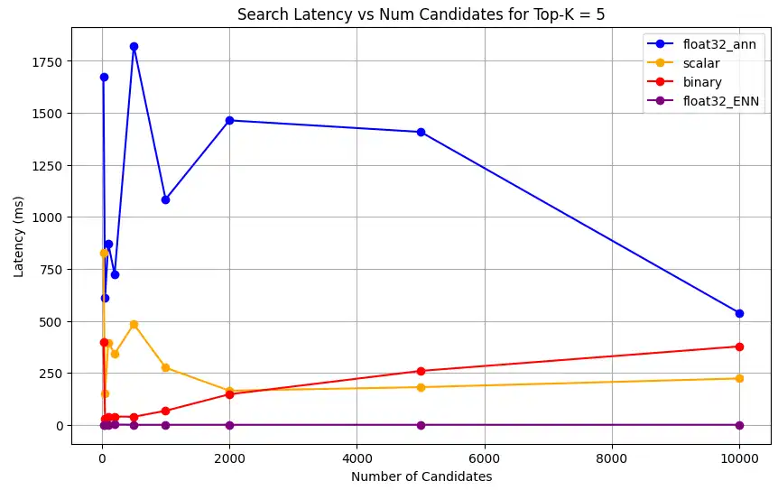
1 # Run the measurements 2 user_query = "How do I increase my productivity for maximum output" 3 top_k_values = [5, 10, 50, 100] 4 num_candidates_values = [25, 50, 100, 200, 500, 1000, 2000, 5000, 10000] 5 6 latency_results = [] 7 8 for vector_search_index in vector_search_indices: 9 latency_results.append( 10 measure_latency_with_varying_topk( 11 user_query, 12 wiki_data_collection, 13 vector_search_index_name=vector_search_index, 14 use_full_precision=False, 15 top_k_values=top_k_values, 16 num_candidates_values=num_candidates_values, 17 ) 18 ) 19 20 # Conduct vector search operation using full precision 21 latency_results.append( 22 measure_latency_with_varying_topk( 23 user_query, 24 wiki_data_collection, 25 vector_search_index_name="vector_index_scalar_quantized", 26 use_full_precision=True, 27 top_k_values=top_k_values, 28 num_candidates_values=num_candidates_values, 29 ) 30 ) 31 32 # Combine all results into a single DataFrame 33 all_latency_results = pd.concat([pd.DataFrame(latency_results)]) Top-K: 5, NumCandidates: 25, Latency: 1672.855906 ms, Precision: _float32_ann ... Top-K: 100, NumCandidates: 10000, Latency: 184.905389 ms, Precision: _float32_ann Top-K: 5, NumCandidates: 25, Latency: 828.45855 ms, Precision: _scalar_ ... Top-K: 100, NumCandidates: 10000, Latency: 214.199836 ms, Precision: _scalar_ Top-K: 5, NumCandidates: 25, Latency: 400.160243 ms, Precision: _binary_ ... Top-K: 100, NumCandidates: 10000, Latency: 360.908558 ms, Precision: _binary_ Top-K: 5, NumCandidates: 25, Latency: 0.239107 ms, Precision: _float32_ENN ... Top-K: 100, NumCandidates: 10000, Latency: 0.179203 ms, Precision: _float32_ENN 지연 시간 측정은 정밀도 유형 전반에 걸쳐 명확한 성능 계층 구조를 보여줍니다. 바이너리 양자화는 가장 빠른 검색 시간을 보여주며, 그 뒤를 스칼라 양자화가 잇습니다. 전체 정밀도 float32 근사 최근접 이웃 작업은 현저하게 높은 지연 시간을 나타냅니다. 양자화 검색과 전체 정밀도 검색 간의 성능 차이는 Top-K 값이 증가할수록 더욱 두드러집니다. float32 등가 최근접 이웃 작업은 가장 느리지만 가장 높은 정밀도의 결과를 제공합니다.
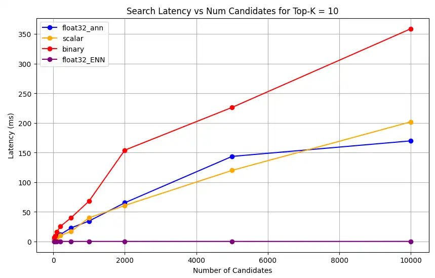
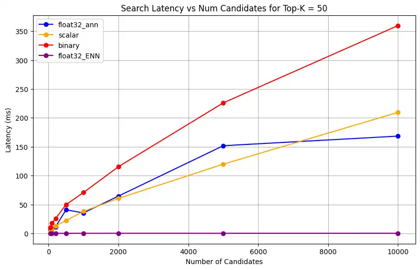
다양한 top-k 값에 대해 검색 지연 시간을 그래프로 나타냅니다.
1 import matplotlib.pyplot as plt 2 3 # Map your precision field to the labels and colors you want in the legend 4 precision_label_map = { 5 "_scalar_": "scalar", 6 "_binary_": "binary", 7 "_float32_ann": "float32_ann", 8 "_float32_ENN": "float32_ENN", 9 } 10 11 precision_color_map = { 12 "_scalar_": "orange", 13 "_binary_": "red", 14 "_float32_ann": "blue", 15 "_float32_ENN": "purple", 16 } 17 18 # Flatten all measurements and find the unique top_k values 19 all_measurements = [m for precision_list in latency_results for m in precision_list] 20 unique_topk = sorted(set(m["top_k"] for m in all_measurements)) 21 22 # For each top_k, create a separate plot 23 for k in unique_topk: 24 plt.figure(figsize=(10, 6)) 25 26 # For each precision type, filter out measurements for the current top_k value 27 for measurements in latency_results: 28 # Filter measurements with top_k equal to the current k 29 filtered = [m for m in measurements if m["top_k"] == k] 30 if not filtered: 31 continue 32 33 # Extract x (num_candidates) and y (latency) values 34 x = [m["num_candidates"] for m in filtered] 35 y = [m["latency_ms"] for m in filtered] 36 37 # Determine the precision, label, and color from the first measurement in this filtered list 38 precision = filtered[0]["precision"] 39 label = precision_label_map.get(precision, precision) 40 color = precision_color_map.get(precision, "blue") 41 42 # Plot the line for this precision type 43 plt.plot(x, y, marker="o", color=color, label=label) 44 45 # Label axes and add title including the top_k value 46 plt.xlabel("Number of Candidates") 47 plt.ylabel("Latency (ms)") 48 plt.title(f"Search Latency vs Num Candidates for Top-K = {k}") 49 50 # Add a legend and grid, then show the plot 51 plt.legend() 52 plt.grid(True) 53 plt.show() 코드는 다음과 같은 지연 시간 차트를 반환합니다. 이 차트들은 벡터 검색의 문서 검색이 이진, 스칼라, float32 등 다양한 임베딩 정밀도에서
top-k(조회된 결과의 수)가 증가할 때 성능이 어떻게 달라지는지 보여줍니다.


표현 용량과 유지율을 측정합니다.
다음 쿼리 MongoDB Vector Search가 실측값 데이터 세트에서 관련 문서를 얼마나 효과적으로 검색하는지 측정합니다. 실측값(Found/Total)에서 총 관련 문서 수 대비 올바르게 발견된 관련 문서의 비율로 계산됩니다. 예시 들어 쿼리 에 실측값에 5 개의 관련 문서가 있고 MongoDB Vector Search가 그 중 4 개를 찾으면 리콜은 0.8 가 됩니다. 또는 80%.
벡터 검색 연산의 표현 용량과 유지율을 측정하는 함수를 정의합니다. 이 함수는 다음을 수행합니다.
전체 정밀도 float32 벡터와 등가 최근접 이웃 검색을 사용하여 기준 검색을 생성합니다.
양자화된 벡터와 근사 최근접 이웃(ANN) 검색을 사용하여 양자화 검색을 수행합니다.
기준 검색 대비 양자화된 검색의 유지율을 계산합니다.
양자화 검색의 경우, 보존률은 합리적인 범위 내에서 유지되어야 합니다. 표현 용량이 낮으면 벡터 검색 작업이 쿼리의 의미적 의미를 포착하지 못해 결과가 정확하지 않을 수 있습니다. 이는 양자화가 효과적이지 않으며, 양자화 과정에 사용된 초기 임베딩 모델이 효과적이지 않음을 나타냅니다. 양자화 인식(quantization-aware) 임베딩 모델을 사용하는 것을 권장합니다. 즉, 학습 과정에서 모델이 양자화 이후에도 의미론적 특성을 유지하는 임베딩을 생성하도록 특별히 최적화된 모델을 의미합니다.
1 def measure_representational_capacity_retention_against_float_enn( 2 ground_truth_collection, 3 collection, 4 quantized_index_name, # This is used for both the quantized search and (with use_full_precision=True) for the baseline. 5 top_k_values, # List/array of top-k values to test. 6 num_candidates_values, # List/array of num_candidates values to test. 7 num_queries_to_test=1, 8 ): 9 retention_results = {"per_query_retention": {}} 10 overall_retention = {} # overall_retention[top_k][num_candidates] = [list of retention values] 11 12 # Initialize overall retention structure 13 for top_k in top_k_values: 14 overall_retention[top_k] = {} 15 for num_candidates in num_candidates_values: 16 if num_candidates < top_k: 17 continue 18 overall_retention[top_k][num_candidates] = [] 19 20 # Extract and store the precision name from the quantized index name. 21 precision_name = quantized_index_name.split("vector_index")[1] 22 precision_name = precision_name.replace("quantized", "").capitalize() 23 retention_results["precision_name"] = precision_name 24 retention_results["top_k_values"] = top_k_values 25 retention_results["num_candidates_values"] = num_candidates_values 26 27 # Load ground truth annotations 28 ground_truth_annotations = list( 29 ground_truth_collection.find().limit(num_queries_to_test) 30 ) 31 print(f"Loaded {len(ground_truth_annotations)} ground truth annotations") 32 33 # Process each ground truth annotation 34 for annotation in ground_truth_annotations: 35 # Use the ground truth wiki_id from the annotation. 36 ground_truth_wiki_id = annotation["wiki_id"] 37 38 # Process only queries that are questions. 39 for query_type, queries in annotation["queries"].items(): 40 if query_type.lower() not in ["question", "questions"]: 41 continue 42 43 for query in queries: 44 # Prepare nested dict for this query 45 if query not in retention_results["per_query_retention"]: 46 retention_results["per_query_retention"][query] = {} 47 48 # For each valid combination of top_k and num_candidates 49 for top_k in top_k_values: 50 if top_k not in retention_results["per_query_retention"][query]: 51 retention_results["per_query_retention"][query][top_k] = {} 52 for num_candidates in num_candidates_values: 53 if num_candidates < top_k: 54 continue 55 56 # Baseline search: full precision using ENN (Float32) 57 baseline_result = custom_vector_search( 58 user_query=query, 59 collection=collection, 60 embedding_path="embedding", 61 vector_search_index_name=quantized_index_name, 62 top_k=top_k, 63 num_candidates=num_candidates, 64 use_full_precision=True, 65 ) 66 baseline_ids = { 67 res["wiki_id"] for res in baseline_result["results"] 68 } 69 70 # Quantized search: 71 quantized_result = custom_vector_search( 72 user_query=query, 73 collection=collection, 74 embedding_path="embedding", 75 vector_search_index_name=quantized_index_name, 76 top_k=top_k, 77 num_candidates=num_candidates, 78 use_full_precision=False, 79 ) 80 quantized_ids = { 81 res["wiki_id"] for res in quantized_result["results"] 82 } 83 84 # Compute retention for this combination 85 if baseline_ids: 86 retention = len( 87 baseline_ids.intersection(quantized_ids) 88 ) / len(baseline_ids) 89 else: 90 retention = 0 91 92 # Store the results per query 93 retention_results["per_query_retention"][query].setdefault( 94 top_k, {} 95 )[num_candidates] = { 96 "ground_truth_wiki_id": ground_truth_wiki_id, 97 "baseline_ids": sorted(baseline_ids), 98 "quantized_ids": sorted(quantized_ids), 99 "retention": retention, 100 } 101 overall_retention[top_k][num_candidates].append(retention) 102 103 print( 104 f"Query: '{query}' | top_k: {top_k}, num_candidates: {num_candidates}" 105 ) 106 print(f" Ground Truth wiki_id: {ground_truth_wiki_id}") 107 print(f" Baseline IDs (Float32): {sorted(baseline_ids)}") 108 print( 109 f" Quantized IDs: {precision_name}: {sorted(quantized_ids)}" 110 ) 111 print(f" Retention: {retention:.4f}\n") 112 113 # Compute overall average retention per combination 114 avg_overall_retention = {} 115 for top_k, cand_dict in overall_retention.items(): 116 avg_overall_retention[top_k] = {} 117 for num_candidates, retentions in cand_dict.items(): 118 if retentions: 119 avg = sum(retentions) / len(retentions) 120 else: 121 avg = 0 122 avg_overall_retention[top_k][num_candidates] = avg 123 print( 124 f"Overall Average Retention for top_k {top_k}, num_candidates {num_candidates}: {avg:.4f}" 125 ) 126 127 retention_results["average_retention"] = avg_overall_retention 128 return retention_results MongoDB Vector Search 인덱스의 성능을 평가하고 비교합니다.
1 overall_recall_results = [] 2 top_k_values = [5, 10, 50, 100] 3 num_candidates_values = [25, 50, 100, 200, 500, 1000, 5000] 4 num_queries_to_test = 1 5 6 for vector_search_index in vector_search_indices: 7 overall_recall_results.append( 8 measure_representational_capacity_retention_against_float_enn( 9 ground_truth_collection=wiki_annotation_data_collection, 10 collection=wiki_data_collection, 11 quantized_index_name=vector_search_index, 12 top_k_values=top_k_values, 13 num_candidates_values=num_candidates_values, 14 num_queries_to_test=num_queries_to_test, 15 ) 16 ) Loaded 1 ground truth annotations Query: 'What happened in 2022?' | top_k: 5, num_candidates: 25 Ground Truth wiki_id: 69407798 Baseline IDs (Float32): [52251217, 60254944, 64483771, 69094871] Quantized IDs: _float32_ann: [60254944, 64483771, 69094871] Retention: 0.7500 ... Query: 'What happened in 2022?' | top_k: 5, num_candidates: 5000 Ground Truth wiki_id: 69407798 Baseline IDs (Float32): [52251217, 60254944, 64483771, 69094871] Quantized IDs: _float32_ann: [52251217, 60254944, 64483771, 69094871] Retention: 1.0000 Query: 'What happened in 2022?' | top_k: 10, num_candidates: 25 Ground Truth wiki_id: 69407798 Baseline IDs (Float32): [52251217, 60254944, 64483771, 69094871, 69265870] Quantized IDs: _float32_ann: [60254944, 64483771, 65225795, 69094871, 70149799] Retention: 1.0000 ... Query: 'What happened in 2022?' | top_k: 10, num_candidates: 5000 Ground Truth wiki_id: 69407798 Baseline IDs (Float32): [52251217, 60254944, 64483771, 69094871, 69265870] Quantized IDs: _float32_ann: [52251217, 60254944, 64483771, 69094871, 69265870] Retention: 1.0000 Query: 'What happened in 2022?' | top_k: 50, num_candidates: 50 Ground Truth wiki_id: 69407798 Baseline IDs (Float32): [25391, 832774, 8351234, 18426568, 29868391, 52241897, 52251217, 60254944, 63422045, 64483771, 65225795, 69094871, 69265859, 69265870, 70149799, 70157964] Quantized IDs: _float32_ann: [25391, 8351234, 29868391, 40365067, 52241897, 52251217, 60254944, 64483771, 65225795, 69094871, 69265859, 69265870, 70149799, 70157964] Retention: 0.8125 ... Query: 'What happened in 2022?' | top_k: 50, num_candidates: 5000 Ground Truth wiki_id: 69407798 Baseline IDs (Float32): [25391, 832774, 8351234, 18426568, 29868391, 52241897, 52251217, 60254944, 63422045, 64483771, 65225795, 69094871, 69265859, 69265870, 70149799, 70157964] Quantized IDs: _float32_ann: [25391, 832774, 8351234, 18426568, 29868391, 52241897, 52251217, 60254944, 63422045, 64483771, 65225795, 69094871, 69265859, 69265870, 70149799, 70157964] Retention: 1.0000 Query: 'What happened in 2022?' | top_k: 100, num_candidates: 100 Ground Truth wiki_id: 69407798 Baseline IDs (Float32): [16642, 22576, 25391, 547384, 737930, 751099, 832774, 8351234, 17742072, 18426568, 29868391, 40365067, 52241897, 52251217, 52851695, 53992315, 57798792, 60163783, 60254944, 62750956, 63422045, 64483771, 65225795, 65593860, 69094871, 69265859, 69265870, 70149799, 70157964] Quantized IDs: _float32_ann: [22576, 25391, 243401, 547384, 751099, 8351234, 17742072, 18426568, 29868391, 40365067, 47747350, 52241897, 52251217, 52851695, 53992315, 57798792, 60254944, 64483771, 65225795, 69094871, 69265859, 69265870, 70149799, 70157964] Retention: 0.7586 ... Query: 'What happened in 2022?' | top_k: 100, num_candidates: 5000 Ground Truth wiki_id: 69407798 Baseline IDs (Float32): [16642, 22576, 25391, 547384, 737930, 751099, 832774, 8351234, 17742072, 18426568, 29868391, 40365067, 52241897, 52251217, 52851695, 53992315, 57798792, 60163783, 60254944, 62750956, 63422045, 64483771, 65225795, 65593860, 69094871, 69265859, 69265870, 70149799, 70157964] Quantized IDs: _float32_ann: [16642, 22576, 25391, 547384, 737930, 751099, 832774, 8351234, 17742072, 18426568, 29868391, 40365067, 52241897, 52251217, 52851695, 53992315, 57798792, 60163783, 60254944, 62750956, 63422045, 64483771, 65225795, 65593860, 69094871, 69265859, 69265870, 70149799, 70157964] Retention: 1.0000 Overall Average Retention for top_k 5, num_candidates 25: 0.7500 ... 출력 결과에는 기준(참값) 데이터셋 내 각 쿼리에 대한 유지율 결과가 표시됩니다 보존율은 0과 1 사이의 소수로 표현되며 1.0은 모든 참값 ID가 유지됨을 의미하고 0.25는 참값 ID의 25%만 유지됨을 의미합니다.
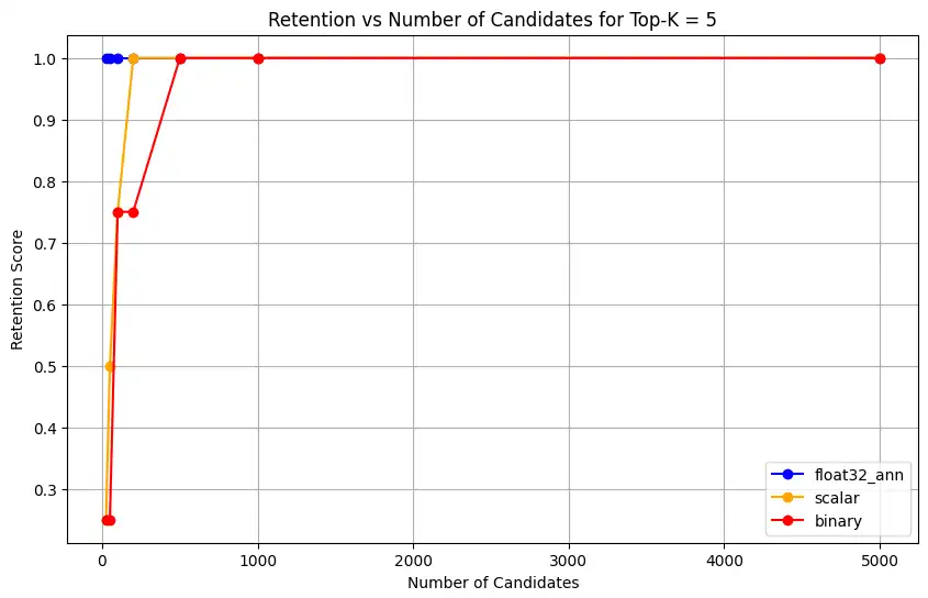
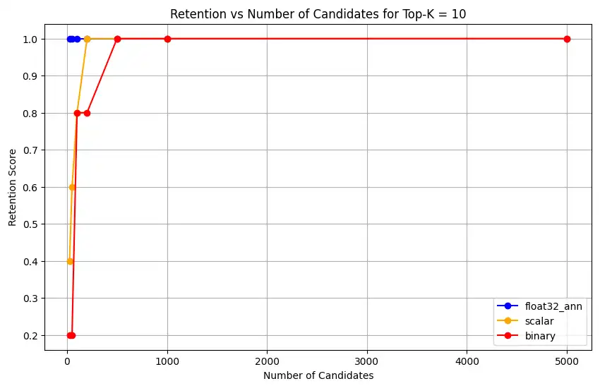
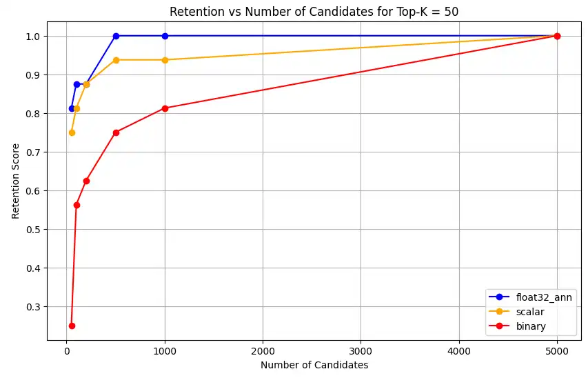
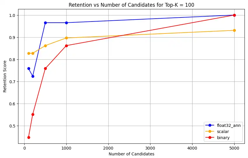
다양한 정밀도 유형의 정확도 보존 능력을 그래프로 나타내세요.
1 import matplotlib.pyplot as plt 2 3 # Define colors and labels for each precision type 4 precision_colors = {"_scalar_": "orange", "_binary_": "red", "_float32_": "green"} 5 6 if overall_recall_results: 7 # Determine unique top_k values from the first result's average_retention keys 8 unique_topk = sorted(list(overall_recall_results[0]["average_retention"].keys())) 9 10 for k in unique_topk: 11 plt.figure(figsize=(10, 6)) 12 # For each precision type, plot retention vs. number of candidates at this top_k 13 for result in overall_recall_results: 14 precision_name = result.get("precision_name", "unknown") 15 color = precision_colors.get(precision_name, "blue") 16 # Get candidate values from the average_retention dictionary for top_k k 17 candidate_values = sorted(result["average_retention"][k].keys()) 18 retention_values = [ 19 result["average_retention"][k][nc] for nc in candidate_values 20 ] 21 22 plt.plot( 23 candidate_values, 24 retention_values, 25 marker="o", 26 label=precision_name.strip("_"), 27 color=color, 28 ) 29 30 plt.xlabel("Number of Candidates") 31 plt.ylabel("Retention Score") 32 plt.title(f"Retention vs Number of Candidates for Top-K = {k}") 33 plt.legend() 34 plt.grid(True) 35 plt.show() 36 37 # Print detailed average retention results 38 print("\nDetailed Average Retention Results:") 39 for result in overall_recall_results: 40 precision_name = result.get("precision_name", "unknown") 41 print(f"\n{precision_name} Embedding:") 42 for k in sorted(result["average_retention"].keys()): 43 print(f"\nTop-K: {k}") 44 for nc in sorted(result["average_retention"][k].keys()): 45 ret = result["average_retention"][k][nc] 46 print(f" NumCandidates: {nc}, Retention: {ret:.4f}") 코드는 다음에 대한 유지율 차트를 반환합니다.
float32_ann,scalar,binary임베딩에 대해 코드는 다음과 유사한 상세 평균 보존률 결과도 반환합니다.Detailed Average Retention Results: _float32_ann Embedding: Top-K: 5 NumCandidates: 25, Retention: 1.0000 NumCandidates: 50, Retention: 1.0000 NumCandidates: 100, Retention: 1.0000 NumCandidates: 200, Retention: 1.0000 NumCandidates: 500, Retention: 1.0000 NumCandidates: 1000, Retention: 1.0000 NumCandidates: 5000, Retention: 1.0000 Top-K: 10 NumCandidates: 25, Retention: 1.0000 NumCandidates: 50, Retention: 1.0000 NumCandidates: 100, Retention: 1.0000 NumCandidates: 200, Retention: 1.0000 NumCandidates: 500, Retention: 1.0000 NumCandidates: 1000, Retention: 1.0000 NumCandidates: 5000, Retention: 1.0000 Top-K: 50 NumCandidates: 50, Retention: 0.8125 NumCandidates: 100, Retention: 0.8750 NumCandidates: 200, Retention: 0.8750 NumCandidates: 500, Retention: 1.0000 NumCandidates: 1000, Retention: 1.0000 NumCandidates: 5000, Retention: 1.0000 Top-K: 100 NumCandidates: 100, Retention: 0.7586 NumCandidates: 200, Retention: 0.7241 NumCandidates: 500, Retention: 0.9655 NumCandidates: 1000, Retention: 0.9655 NumCandidates: 5000, Retention: 1.0000 _scalar_ Embedding: Top-K: 5 NumCandidates: 25, Retention: 0.2500 NumCandidates: 50, Retention: 0.5000 NumCandidates: 100, Retention: 0.7500 NumCandidates: 200, Retention: 1.0000 NumCandidates: 500, Retention: 1.0000 NumCandidates: 1000, Retention: 1.0000 NumCandidates: 5000, Retention: 1.0000 Top-K: 10 NumCandidates: 25, Retention: 0.4000 NumCandidates: 50, Retention: 0.6000 NumCandidates: 100, Retention: 0.8000 NumCandidates: 200, Retention: 1.0000 NumCandidates: 500, Retention: 1.0000 NumCandidates: 1000, Retention: 1.0000 NumCandidates: 5000, Retention: 1.0000 Top-K: 50 NumCandidates: 50, Retention: 0.7500 NumCandidates: 100, Retention: 0.8125 NumCandidates: 200, Retention: 0.8750 NumCandidates: 500, Retention: 0.9375 NumCandidates: 1000, Retention: 0.9375 NumCandidates: 5000, Retention: 1.0000 Top-K: 100 NumCandidates: 100, Retention: 0.8276 NumCandidates: 200, Retention: 0.8276 NumCandidates: 500, Retention: 0.8621 NumCandidates: 1000, Retention: 0.8966 NumCandidates: 5000, Retention: 0.9310 _binary_ Embedding: Top-K: 5 NumCandidates: 25, Retention: 0.2500 NumCandidates: 50, Retention: 0.2500 NumCandidates: 100, Retention: 0.7500 NumCandidates: 200, Retention: 0.7500 NumCandidates: 500, Retention: 1.0000 NumCandidates: 1000, Retention: 1.0000 NumCandidates: 5000, Retention: 1.0000 Top-K: 10 NumCandidates: 25, Retention: 0.2000 NumCandidates: 50, Retention: 0.2000 NumCandidates: 100, Retention: 0.8000 NumCandidates: 200, Retention: 0.8000 NumCandidates: 500, Retention: 1.0000 NumCandidates: 1000, Retention: 1.0000 NumCandidates: 5000, Retention: 1.0000 Top-K: 50 NumCandidates: 50, Retention: 0.2500 NumCandidates: 100, Retention: 0.5625 NumCandidates: 200, Retention: 0.6250 NumCandidates: 500, Retention: 0.7500 NumCandidates: 1000, Retention: 0.8125 NumCandidates: 5000, Retention: 1.0000 Top-K: 100 NumCandidates: 100, Retention: 0.4483 NumCandidates: 200, Retention: 0.5517 NumCandidates: 500, Retention: 0.7586 NumCandidates: 1000, Retention: 0.8621 NumCandidates: 5000, Retention: 1.0000 리콜(재현율) 결과는 세 가지 임베딩 유형에서 뚜렷한 성능 패턴을 보여줍니다.
스칼라 양자화는 K 값이 높아질수록 검색 정확도가 크게 향상됨을 보여줍니다. 이진 양자화는 초기 성능이 낮으나 Top-K 50 및 100에서 개선되어 계산 효율성과 리콜 성능 간의 절충이 있음을 시사합니다. Float32 임베딩은 초기 성능이 가장 뛰어나며 Top-K 50 및 100에서 스칼라 양자화와 동일한 최대 리콜에 도달합니다.
이는 float32가 낮은 Top-K 값에서 더 나은 재현율을 제공하는 반면 스칼라 양자화는 더 높은 Top-K 값에서 동등한 성능을 달성하면서 계산 효율성도 높일 수 있음을 시사합니다. 이진 양자화는 회수율 한계가 낮음에도 불구하고 메모리나 연산 제약이 최대 회수 정확도보다 더 중요한 상황에서는 여전히 유용할 수 있습니다.