Building Gen AI prototypes is straightforward. Whether you're building search, RAG, or agentic applications, the main focus when prototyping is often accuracy. But production is different. In production, you’re handling thousands or millions of queries instead of a handful of tests. Your users expect accurate responses, and they want them instantly. This requires optimizing for three things at once: accuracy, speed, and operating costs.
In this guide, we will focus on optimizing embedding-based retrieval, a cornerstone of modern search, RAG, and agentic systems. Inefficiencies in your retrieval component can compound quickly since retrieval happens on every query—and often multiple times per query in agentic systems. You’ll learn techniques for optimizing your retrieval pipeline across all three dimensions so you can make data-driven decisions about what makes the most sense for your specific use case. We'll cover:
Asymmetric retrieval using Voyage AI by MongoDB’s Voyage 4 series of embedding models
Dimensionality reduction via Matryoshka Learning
Auto-quantization using MongoDB Atlas
Evaluating the impact of each technique on cost, latency, and accuracy
Overview of optimization techniques
In this guide, we will focus on the following three optimization techniques for embedding-based retrieval:
Asymmetric retrieval
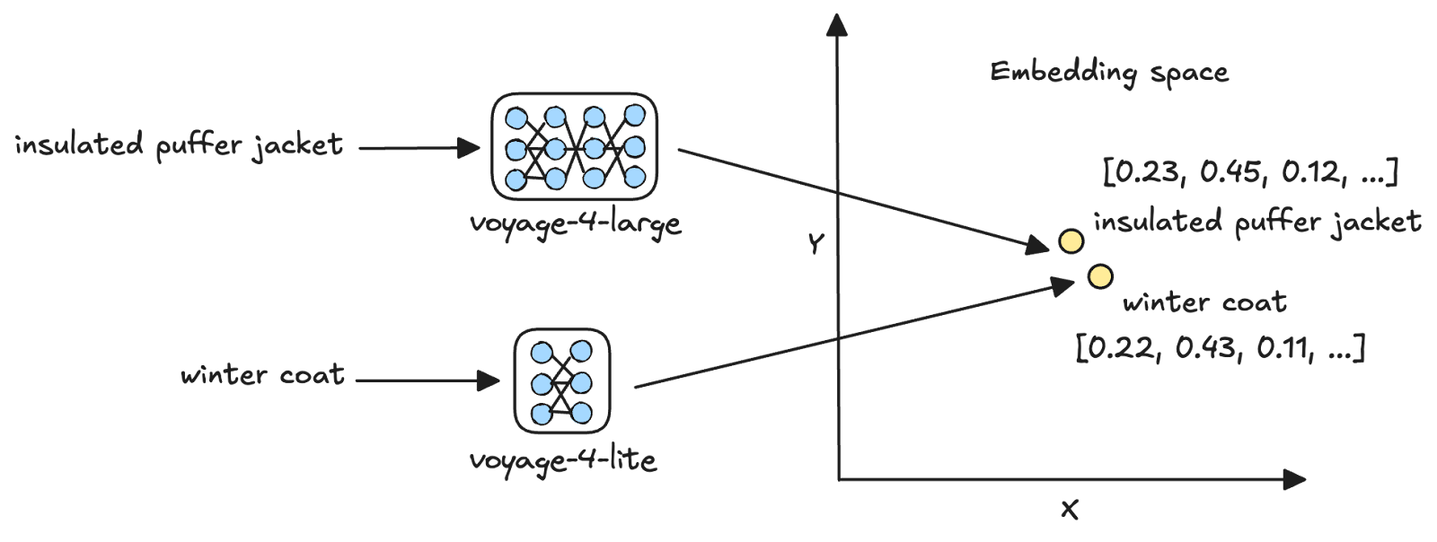
Asymmetric retrieval is the process of vectorizing queries and documents using different embedding models [1]. Voyage AI’s latest Voyage 4 series of embedding models has a shared embedding space, thus facilitating asymmetric retrieval. For example, you can embed user queries using the smallest model in the family, voyage-4-lite, and use it to search for document embeddings generated using the largest, voyage-4-large.
Asymmetric retrieval is most effective when the cost of vectorizing your document corpus is small relative to the cumulative cost of vectorizing queries over time. By vectorizing documents with a larger model and queries with a smaller one, you get the accuracy benefits of the larger model’s vector representations while keeping per-query cost low.
Vector quantization
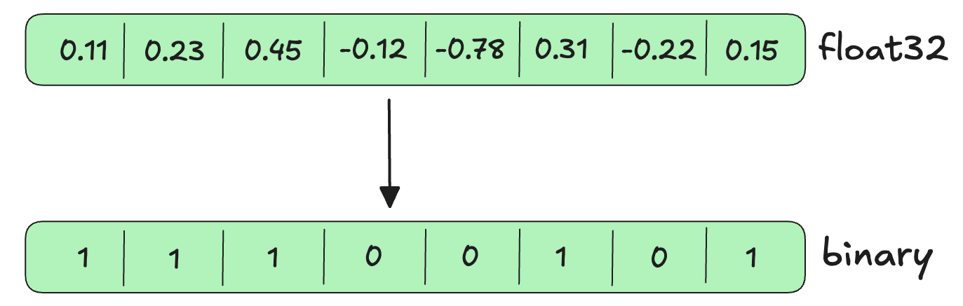
Vector quantization is the process of compressing high-precision vectors into lower-precision formats [2] . For example, scalar quantization converts float32 vectors, which require 32 bits to store each dimension, to int8, which requires only 8 bits per dimension. Binary quantization goes further, converting float32 vectors to binary (0 or 1) values requiring just 1 bit per dimension.
The key benefit of quantization is that it reduces the memory footprint of vector search, thus reducing query latency while preserving most of the retrieval accuracy.
Dimensionality reduction
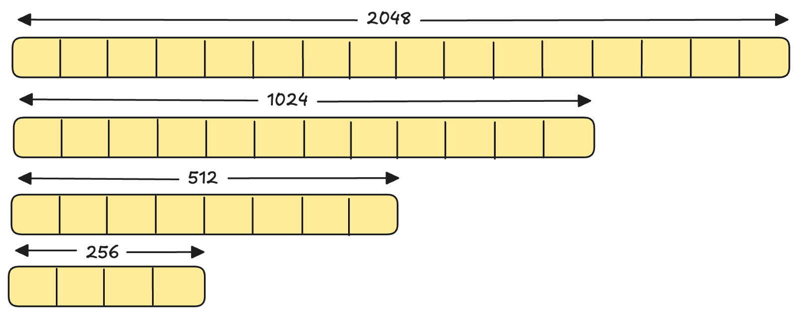
Matryoshka Representation Learning (MRL) is a technique for training embedding models such that earlier dimensions capture more important information and later dimensions capture less important information [3]. This allows you to truncate a single embedding to fewer dimensions while retaining most of the semantic information needed for downstream tasks like retrieval. For example, all models in the Voyage 4 series support 2048, 1024, 512, and 256 dimensions from a single model.
Truncating the embeddings reduces storage costs, lowers memory requirements during search, and improves query latency with minimal impact on retrieval quality.
Optimization framework
Each of the techniques discussed above targets different performance bottlenecks. We will evaluate each of them later in this blog, but here is a framework to choose which techniques to evaluate based on your application’s requirements:
These techniques are complementary and can be combined to minimize storage costs, per-query costs, and query latency, as long as you're satisfied with the accuracy trade-off.
Evaluating different optimization strategies
Let's systematically evaluate each of these techniques on a sample dataset. You can apply this same evaluation methodology to your own data to determine which optimizations make sense for your use case.
About the dataset
We will use the NFCorpus dataset available on Hugging Face. The dataset consists of three components: a corpus of medical documents, sample queries, and relevance judgments that indicate which documents are relevant to each query, along with their relevance scores.
Tip
Relevance judgments are required for measuring retrieval quality metrics such as NDCG, MRR, and recall. While our dataset includes these ground-truth judgments, you will need to create them for your own evaluation dataset. To do this, start with 50 to 100 representative queries, and for each query:
- Manual labeling (most accurate): Have domain experts label the top 20 to 30 documents retrieved by your baseline system as relevant or not, or use a scale such as 0 to 2.
- LLM-assisted labeling (quick but imperfect): Use an LLM to generate relevance scores based on a rubric you specify and then validate a sample manually to ensure correctness.
Where’s the code
The Jupyter Notebook for this tutorial is available on GitHub in our GenAI Showcase repository. To follow along, run the notebook in Google Colab (or a similar environment) and refer to this tutorial for explanations of key code blocks.
Step 1: Install required libraries
Begin by installing the following libraries:
voyageai: Voyage AI's Python SDK
pymongo: MongoDB's Python driver
datasets: Python library to interact with datasets on Hugging Face
scikit-learn: Python library consisting of modules for machine learning and data mining
Step 2: Setup prerequisites
You will use models from Voyage AI’s latest Voyage 4 series and MongoDB as the vector database for this evaluation. First, create a MongoDB Atlas database cluster, obtain its connection string, and get a Voyage API key from within your cluster. Follow these steps to get set up:
Register for a free MongoDB Atlas account.
Obtain the connection string for your database cluster.
- Obtain a Voyage API key in Atlas.
Next, set the API key as an environment variable and initialize the Voyage AI client:
Set the MongoDB connection string and initialize the MongoDB client:
Step 3: Download the dataset
Next, download the NFCorpus datasets from Hugging Face and load them as Pandas dataframes.
Notice that you set the split parameter of the load_dataset method to “corpus” to download the corpus, and to “queries” to download the sample queries. For the relevance judgments, you are downloading only the “test” split to obtain relevance scores for the test queries (the sample queries are split into train, validation, and test subsets).
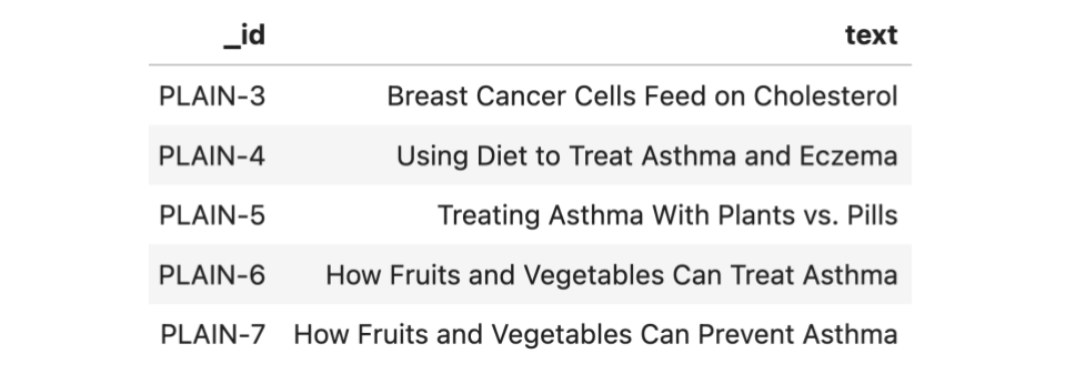
In their current form, each row in the queries dataframe (queries) consists of a query ID (_id) and the query text (text) as follows:
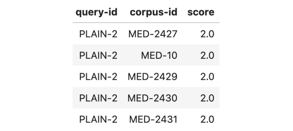
Each row in the relevance judgments dataframe (qrels) consists of a query ID (query-id), a corpus ID (corpus-id) indicating the ID of a document in the corpus, and a score (score) between 0 (not relevant) and 2 (highly relevant), indicating the relevance of the document to the query. A preview of this dataframe is as follows:
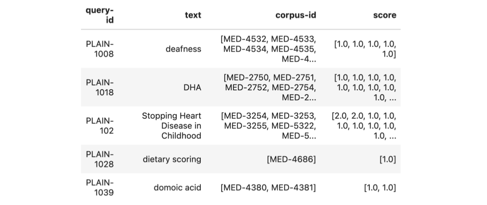
Format the evaluation dataset in a way that’s easy to use downstream:
The above code merges the queries and qrels dataframes, retaining only queries in the test subset. It then groups the resulting dataframe by the query ID and aggregates the relevant corpus IDs and their scores into a list. Each row in the final dataframe consists of a query ID (query-id), the query text (text), the list of relevant document IDs (corpus-id), and their relevance scores (score). Here is a preview of this dataframe:
Step 4: Embed the corpus
Next, generate embeddings for the corpus. You will embed the corpus in batches, so create two helper functions: one to create batches of texts to embed, and another to generate embeddings using the Atlas Embedding and Reranking API.
The above code uses the embed method of the Atlas Embedding and Reranking API to generate text embeddings. The texts parameter of the method indicates the list of texts to embed, the model parameter indicates the name of the model to use for embedding, the input_type parameter can be one of “query” or “document”, depending on what’s being embedded, and the output_dimensions parameter specifies the number of dimensions for the embeddings.
The above function iterates through the corpus in chunks of batch_size, generates embeddings for each batch using the generate_embeddings function, accumulates the embeddings in a list, and returns the complete list.
Now add embeddings with 1024 and 512 dimensions to each document in the corpus, using the voyage-4-large model. This will allow you to compare the impact of dimensionality reduction during our evaluation. Since your corpus is loaded as a dataframe, adding the embeddings is as simple as:
The above code adds two columns to the dataframe, namely 1024_embedding and 512_embedding, consisting of embeddings of 1024 and 512 dimensions, respectively. Finally, convert the corpus dataframe into a list of objects (corpus_dict) to insert into MongoDB using the to_dict() method. A sample object looks like this:
Step 5: Ingest data into MongoDB
Next, ingest the corpus with embeddings into MongoDB:
In the above code, you first access a database named mongodb_eval and a collection named docs within it. Then any existing documents get deleted from the collection using the delete_many method—the {} parameter indicates that all documents must be deleted. Then you bulk-insert the documents you previously created (corpus_dict) into the collection using the insert_many method.
Step 6: Create vector search indexes
To keep evaluation straightforward, create a few different vector search index configurations that will allow you to independently observe the impact of the optimization techniques.
As seen above, you create two vector search indexes, each on the 1024_embedding and 512_embedding fields, one with auto-quantization enabled and another without. Auto-quantization automatically quantizes the embeddings within documents at index creation, and query vectors at query time. To enable vector auto-quantization in MongoDB, simply set the quantization field to scalar or binary in the vector search index definition. You will only evaluate binary quantization in this tutorial.
Now, actually create the indexes. To do this, use the create_search_indexes method in Pymongo, which allows you to create multiple search indexes in a single API call:
Notice the disk size and memory requirements of the indexes created in your MongoDB Atlas cluster:
A few things to note from the above:
The indexes with auto-quantization enabled have a slightly larger disk size but require 96% less RAM than their full-precision counterparts. This is because the full-fidelity vectors are stored on disk alongside the quantized vectors and used to rescore the vector search results. This rescoring ensures that the final search results are highly accurate despite the vector compression.
Dimensionality reduction reduces both the disk space and memory required by 50%.
Combining dimensionality reduction and binary quantization results in a 48% reduction in disk size and 98% reduction in required RAM.
Tip
You can also ingest pre-quantized vectors into MongoDB instead of leveraging auto-quantization. This will reduce storage costs since full-fidelity vectors are not stored. However, this also means there will be no rescoring step, which may result in lower accuracy. Generally, we recommend auto-quantization, as storage is relatively cheap and rescoring improves accuracy.
Step 7: Evaluation
You’ve seen how dimensionality reduction and quantization affect storage and memory requirements, but what about their impact on actual query performance? And how does asymmetric retrieval compare? Let's evaluate each configuration and observe the trade-offs.
First, create a helper function to perform vector search:
The vector_search function above takes a query string (query) and evaluation configuration (config) as input and:
uses the generate_embeddings helper function from step 4 to generate the query embedding, based on the embedding model and dimensions specified in the evaluation config.
defines a MongoDB aggregation pipeline that has two stages:
$vectorSearch: Performs vector search. The queryVector field in this stage contains the embedded user query, the path refers to the path of the embedding field in the documents, numCandidates denotes the number of nearest neighbors to consider in the vector space when performing vector search, and finally, limit indicates the number of documents that will be returned from the vector search.
$project: includes only certain fields (set to the value 1) in the final results. In this case, only the document ID (_id) and the vector search score are returned.
uses the explain command to get the execution statistics for the vector search query, including the execution time.
uses the aggregate method to get the results from performing the vector search query.
Tip
You’re measuring query latency as vector search latency alone, excluding embedding generation time. This is a valid approximation when using the Atlas Embedding and Reranking API, where embedding generation time is similar across models and dimensions. However, if you were self-hosting your embedding models, total query latency would equal embedding latency plus search latency.
Next, define a helper function to evaluate the different optimization options:
The evaluate function above iterates through the test queries and for each query:
uses the vector_search helper function above to get the top 10 most relevant documents and the query execution time.
uses sklearn’s ndcg_score method to calculate the NDCG@10. y_true is the list of ground truth relevance scores of the documents in the top 10 list, while y_score consists of the vector search similarity scores.
calculates the mean NDCG@10, P50 and P95 latency across all the test queries.
The results of the evaluation are as follows:
All three optimizations retain 98-99% of baseline retrieval accuracy. Binary quantization provides the largest improvement in query latency at 60%, followed by dimensionality reduction at 40%. Now, let’s examine asymmetric retrieval more closely, whose primary benefit is reducing query embedding costs at scale.
The above calculations assume an average query length of 30 tokens. Voyage 4 pricing information is linked in the References section. [4]
Asymmetric retrieval results in significant cost savings as your user base grows. Using voyage-4 for query embeddings cuts costs in half, while voyage-4-lite reduces costs by 83%. As your application scales from 10,000 to 1M queries per day, annual savings grow from $11K to over $1M.
A summary of our findings on the evaluation dataset is as follows:
Binary quantization improves query latency by 60% and reduces vector search memory requirements by 96% while maintaining 99% of baseline accuracy.
Dimensionality reduction (1024d to 512d) delivers 40% faster queries and requires 50% less storage and memory while maintaining 98% of baseline accuracy.
Asymmetric retrieval (voyage-4) reduces query embedding costs by 50% with minimal impact on retrieval quality.
Conclusion
In this tutorial, we explored three retrieval optimization techniques—asymmetric retrieval, vector quantization, and dimensionality reduction—to optimize cost, latency, and accuracy in AI applications.
Not every application needs all three optimizations. Evaluate your specific bottlenecks:
If query latency is your primary concern, explore quantization and dimensionality reduction.
If high query volumes drive up your embedding costs, consider asymmetric retrieval.
Measure the trade-offs against your accuracy requirements, then apply only the optimizations your application truly needs.
Next Steps
Register for a Voyage AI account to claim your free 200 million tokens and to try out the Voyage 4 model family. To learn more about the models, visit our API documentation and follow us on X (Twitter) and LinkedIn for more updates.
References
[2] Vector quantization in MongoDB Atlas
[3] Matryoshka Representation Learning
[4] Voyage 4 pricing