MongoDB 3.0 introduces compression with the WiredTiger storage engine. In this post we will take a look at the different options, and show some examples of how the feature works. As always, YMMV, so we encourage you to test your own data and your own application.
Why compression?
Everyone knows storage is cheap, right?
But chances are you’re adding data faster than storage prices are declining, so your net spend on storage is rising. Your internal costs might also incorporate management and other factors, so they may be significantly higher than commodity market prices. In other words, it still pays to look for ways to reduce your storage needs.
Size is one factor, and there are others. Disk I/O latency is dominated by seek time on rotational storage. By decreasing the size of the data, fewer disk seeks will be necessary to retrieve a given quantity of data, and disk I/O throughput will improve. In terms of RAM, some compressed formats can be used without decompressing the data in memory. In these cases more data can fit in RAM, which improves performance.
Storage properties of MongoDB
There are two important features related to storage that affect how space is used in MongoDB: BSON and dynamic schema.
MongoDB stores data in BSON, a binary encoding of JSON-like documents (BSON supports additional data types, such as dates, different types of numbers, binary). BSON is efficient to encode and decode, and it is easily traversable. However, BSON does not compress data, and it is possible its representation of data is actually larger than the JSON equivalent.
One of the things users love about MongoDB’s document data model is dynamic schema. In most databases, the schema is described and maintained centrally in a catalog or system tables. Column names are stored once for all rows. This approach is efficient in terms of space, but it requires all data to be structured according to the schema. In MongoDB there is currently no central catalog: each document is self-describing. New fields can be added to a document without affecting other documents, and without registering the fields in a central catalog.
The tradeoff is that with greater flexibility comes greater use of space. Field names are defined in every document. It is a best practice to use shorter field names when possible. However, it is also important not to take this too far – single letter field names or codes can obscure the field names, making it more difficult to use the data.
Fortunately, traditional schema is not the only way to be space efficient. Compression is very effective for repeating values like field names, as well as much of the data stored in documents.
There is no Universal Compression
Compression is all around us: images (JPEG, GIF), audio (mp3), video (MPEG), and most web servers compress web pages before sending to your browser using gzip. Compression algorithms have been around for decades, and there are competitions that award innovation.
Compression libraries rely on CPU and RAM to compress and decompress data, and each makes different tradeoffs in terms of compression rate, speed, and resource utilization. For example, one measure of today’s best compression library for text can compress 1GB of Wikipedia data to 124MB compared to 323MB for gzip, but it takes about almost 3,000 times longer and 30,000 times more memory to do so. Depending on your data and your application, one library may be much more effective for your needs than others.
MongoDB 3.0 introduces WiredTiger, a new storage engine that supports compression. WiredTiger manages disk I/O using pages. Each page contains many BSON documents. As pages are written to disk they are compressed by default, and when they are read into the cache from disk they are decompressed.
One of the basic concepts of compression is that repeating values – exact values as well as patterns – can be stored once in compressed form, reducing the total amount of space. Larger units of data tend to compress more effectively as there tend to be more repeating values. By compressing at the page level – commonly called block compression – WiredTiger can more efficiently compress data.
WiredTiger supports multiple compression libraries. You can decide which option is best for you at the collection level. This is an important option – your access patterns and your data could be quite different across collections. For example, if you’re using GridFS to store large documents such as images and videos, MongoDB automatically breaks the large files into many smaller “chunks” and reassembles them when requested. The implementation of GridFS maintains two collections: fs.files, which contains the metadata for the large files and their associated chunks, and fs.chunks, which contains the large data broken into 255KB chunks. With images and videos, compression will probably be beneficial for the fs.files collection, but the data contained in fs.chunks is probably already compressed, and so it may make sense to disable compression for this collection.
Compression options in MongoDB 3.0
In MongoDB 3.0, WiredTiger provides three compression options for collections:
- No compression
- Snappy (enabled by default) – very good compression, efficient use of resources
- zlib (similar to gzip) – excellent compression, but more resource intensive
There are two compression options for indexes:
- No compression
- Prefix (enabled by default) – good compression, efficient use of resources
You may wonder why the compression options for indexes are different than those for collections. Prefix compression is fairly simple – the “prefix” of values is deduplicated from the data set. This is especially effective for some data sets, like those with low cardinality (eg, country), or those with repeating values, like phone numbers, social security codes, and geo-coordinates. It is especially effective for compound indexes, where the first field is repeated with all the unique values of second field. Prefix indexes also provide one very important advantage over Snappy or zlib – queries operate directly on the compressed indexes, including covering queries.
When compressed collection data is accessed from disk, it is decompressed in cache. With prefix compression, indexes can remain compressed in RAM. We tend to see very good compression with indexes using prefix compression, which means that in most cases you can fit more of your indexes in RAM without sacrificing performance for reads, and with very modest impact to writes. The compression rate will vary significantly depending on the cardinality of your data and whether you use compound indexes.
Some things to keep in mind that apply to all the compression options in MongoDB 3.0:
- Random data does not compress well
- Binary data does not compress well (it may already be compressed)
- Text compresses especially well
- Field names compress well in documents (the additional benefits of short field names are modest)
Compression is enabled by default for collections and indexes in the WiredTiger storage engine. To explicitly set the compression for the replica at startup, specify the appropriate options in the YAML config file. use the command line option --wiredTigerCollectionBlockCompressor. Because WiredTiger is not the default storage engine in MongoDB 3.0, you’ll also need to specify the --storageEngine option to use WiredTiger and take advantage of these compression features.
To specify compression for specific collections, you’ll need to override the defaults by passing the appropriate options in the db.createCollection() command. For example, to create a collection called email using the zlib compression library:
How to measure compression
The best way to measure compression is to separately load the data with and without compression enabled, then compare the two sizes. The db.stats() command returns many different storage statistics, but the two that matter for this comparison are storageSize and indexSize. Values are returned in bytes, but you can convert to MB by passing in 1024*1024:
This is the method we used for the comparisons provided below.
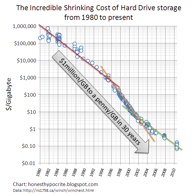
Testing compression on different data sets
Let’s take a look at some different data sets to see how some of the compression options perform. We have four databases:
Enron
This is the infamous Enron email corpus. It includes about a half million emails. There’s a great deal of text in the email body fields, and some of the metadata has low cardinality, which means that they’re both likely to compress well. Here’s an example (the email body is truncated):
Here’s how the different options performed with the Enron database:
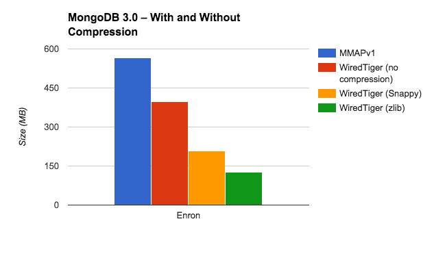
Flights
The US Federal Aviation Administration (FAA) provides data about on-time performance of airlines. Each flight is represented as a document. Many of the fields have low cardinality, so we express this data set to compress well:
Here’s how the different options performed with the Flights database:
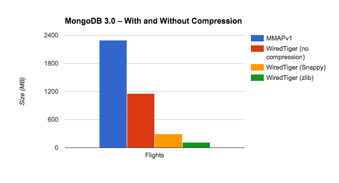
MongoDB Config Database
This is the metadata MongoDB stores in the config database for sharded clusters. The manual describes the various collections in that database. Here’s an example from the chunks collection, which stores a document for each chunk in the cluster:
Here’s how the different options performed with the config database:
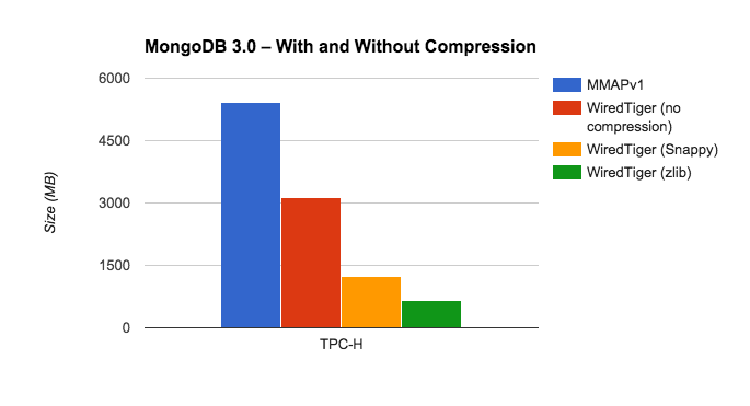
TPC-H
TPC-H is a classic benchmark used for testing relational analytical DBMS. The schema has been modified to use MongoDB’s document model. Here’s an example from the orders table with only the first of many line items displayed for this order:
Here’s how the different options performed with the TPC-H database:
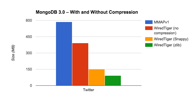
Twitter
This is a database of 200K tweets. Here’s a simulated tweet introducing our Java 3.0 driver:
Here’s how the different options performed with the Twitter database:
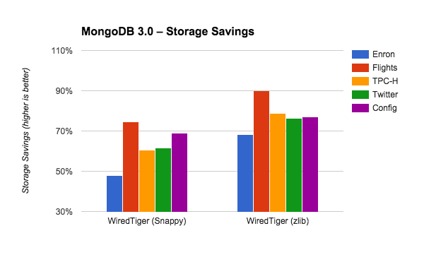
Comparing compression rates
The varying sizes of these databases make them difficult to compare side by side in terms of absolute size. We can take a closer look at the benefits by comparing the storage savings provided by each option. To do this, we compare the size of each database using Snappy and zlib to the uncompressed size in WiredTiger. As above, we’re adding the value of storageSize and indexSize.
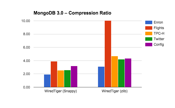
Another way some people describe the benefits of compression is in terms of the ratio of the uncompressed size to the compressed size. Here’s how Snappy and zlib perform across the five databases.
How to test your own data
There are two simple ways for you to test compression with your data in MongoDB 3.0.
If you’ve already upgraded to MongoDB 3.0, you can simply add a new secondary to your replica set with the option to use the WiredTiger storage engine specified at startup. While you’re at it, make this replica hidden with 0 votes so that it won’t affect your deployment. This new replica set member will perform an initial sync with one of your existing secondaries. After the initial sync is complete, you can remove the WiredTiger replica from your replica set then connect to that standalone to compare the size of your databases as described above. For each compression option you want to test, you can repeat this process.
Another option is to take a mongodump of your data and use that to restore it into a standalone MongoDB 3.0 instance. By default your collections will use the Snappy compression option, but you can specify different options by first creating the collections with the appropriate setting before running mongorestore, or by starting mongod with different compression options. This approach has the advantage of being able to dump/restore only specific databases, collections, or subsets of collections to perform your testing.
For examples of syntax for setting compression options, see the section “How to use compression.”
A note on capped collections
Capped collections are implemented very differently in the MMAP storage engines as compared to WiredTiger (and RocksDB). In MMAP space is allocated for the capped collection at creation time, whereas for WiredTiger and RocksDB space is only allocated as data is added to the capped collection. If you have many empty or mostly-empty capped collections, comparisons between the different storage engines may be somewhat misleading for this reason.
If you’re considering updating your version of MongoDB, take a look at our Major Version Upgrade consulting services:
UPGRADE WITH CONFIDENCEAsya is Lead Product Manager at MongoDB. She joined MongoDB as one of the company's first Solutions Architects. Prior to MongoDB, Asya spent seven years in similar positions at Coverity, a leading development testing company. Before that she spent twelve years working with databases as a developer, DBA, data architect and data warehousing specialist.