Implementing an Online Parquet Shredder
April 11, 2023 | Updated: June 23, 2025
In Atlas Data Federation (ADF) we’ve found that many customers want to take their data, say from an Atlas cluster, and emit to their own blob storage as a parquet file. This is a popular and–for many customers–important feature we’re proud to provide. Converting data from our native BSON format, complete with flexible-schema and row-based representation, to the fixed-schema, columnar parquet format without compromises is not a computationally easy task. We’ve provided this to customers for years now, but with our February 21st release we’re excited to announce the release of a much-improved BSON-to-Parquet writer.
Among behind-the-scenes changes, one exciting improvement that will be immediately visible to customers is that the efficiency of our parquet-writer is substantively improved both for CPU and memory-usage. From our internal benchmarks we see a 2x improvement in throughput, and our production metrics indicate that about bears out for our customer workloads, of course with some variance. We have only ever seen throughput improvements; we have not found a single workload that has worse performance.
In this blog post I’ll share a high-level view of the core technical challenge and how we built together at MongoDB to create this solution.
The technical challenge
If you use ADF and issue an aggregate that ends with an $out stage and the parquet format specified, we’ll take the result of that aggregation and emit it to a parquet file in the named blob storage. We can imagine an aggregate’s result as a stream of BSON documents. The role ADF plays, then, is to take that document-stream, convert it to a parquet file, and place it in the blob storage. Smoothing away the rough details, we’re left with the core technical challenge:
We want to convert a stream of row-based, flexible-schema BSON documents into a columnar, fixed-schema parquet file.
That’s quite a challenge!
Our initial approach
Our past approach understandably focused on stability and simplicity over everything else. We built out our initial parquet offering by leveraging existing, production-tested subcomponents. In broad strokes, it did the following:
-
Scan through the entire document stream to build the global schema that describes them all.
-
Open a parquet file with that schema, and then scan through the documents again, “shredding” their contents one-by-one into the parquet file’s columns.
This two-pass algorithm worked and served our customers, but has two fundamental drawbacks. The most immediate drawback is exactly that it is two-pass, and the second pass has to entirely wait on the first: we’re unable to create a parquet file until we know the schema, and we can’t be certain of what the schema is until we’ve seen the last document (for example, the last document may introduce a new field). The second drawback is how, when we shred our documents, we’re placing them directly in the file. A consequence of this is that, absent significant re-engineering, it is very difficult to flush the contents to disk until the file is complete.1
As we saw customers using $out-to-parquet more and more, we knew it would be worth the investment to shift to more performant machinery.
Changes for our new approach
Our new approach introduces what we call the Online Shredder. This algorithm enables us to effectively shred a stream of documents into a columnar format in a single pass, building the schema in parallel. It doesn’t shred immediately into a parquet file, but instead to an intermediate file that enables us to more easily swap memory to disk. Finally, we’re excited to leverage the apache-go parquet writer. We’ve found it to be an exceptionally performant and feature-rich library. Most of the rest of this blog post is a high-level description of the design and implementation of the online shredder that supports this new approach.
The new approach in-depth
We have a stream of documents, and we want to shred them into a columnar form. The overall challenge behind this operation is supporting MongoDB’s flexible schema and maintaining the right information for lossless parquet emission. In particular, the “language barrier” between MongoDB’s row-based, flexible schema and Parquet’s column-based, fixed schema introduces 3 hurdles:
-
Missing or New Fields: One document may have a field, and then a later document doesn’t include that field. Or, we may have a new document that for the first-time-ever introduces a new field.
-
Polymorphism: Two documents may have a field with the same namepath, but different types.
-
Structural Metadata: Parquet enables reassembly of its records using metadata that encodes information derived from the global schema. With our online approach, we have to commit to this metadata without yet fully knowing the global schema.
We’ll describe the design of the online shredder first by explaining how it builds a schema as it scans over the document. Then we’ll build off of those concepts and extend them to not just build the schema, but shred the documents into an in-memory columnar representation. We will see that the technical challenge in shredding comes from efficiently maintaining the structural metadata. The punchline will be that careful application of invariants from our schema-building gives us an elegant approach to maintaining this metadata.
Introducing the schema
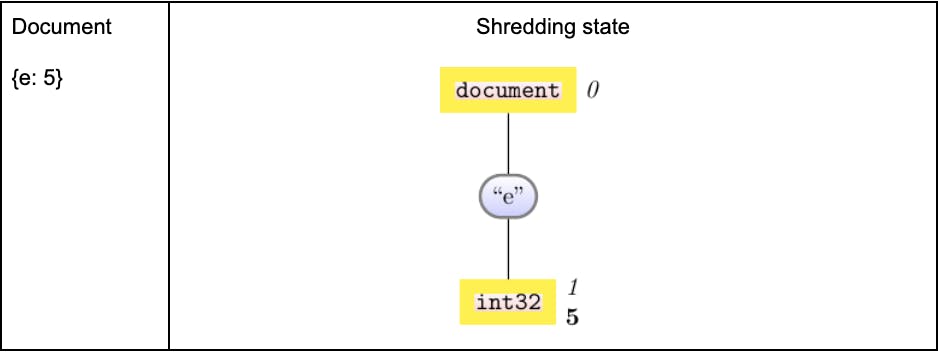
Our document stream may contain documents that vary wildly in structure. For example, say the collection we want to emit as Parquet has these 4 documents
-
{e: 5}
-
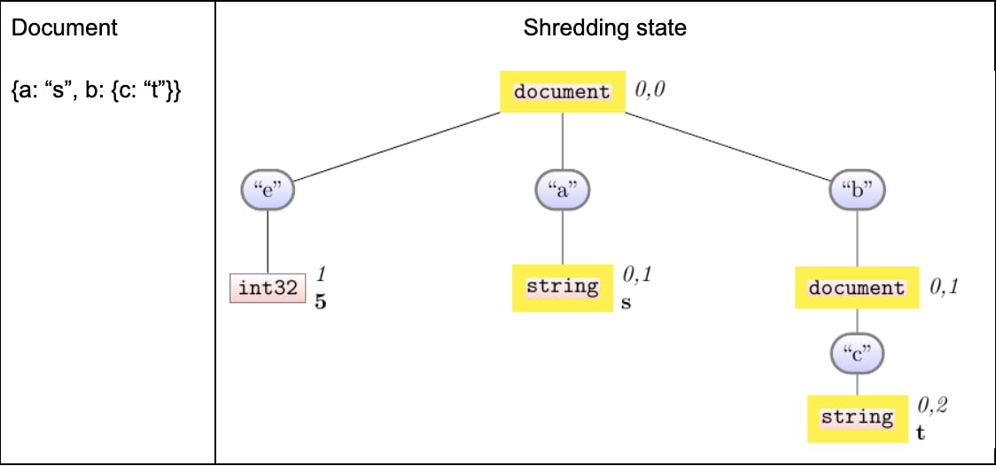
{a: “s”, b: {c: “t”}}
-
{}
-
{a: 8, b: {c: “r”, d: true}}
To put these 4 documents in the same file, parquet requires they all be described by the same schema. For our purposes we can understand a schema as a sort of meta-document: a document with key-value pairs, but with special meta-values. Concretely, here are the individual schemas for those four documents:
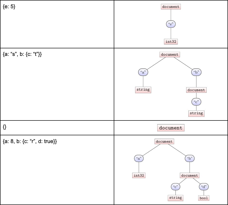
The nested sub-document under b in the second and fourth documents illustrate how a schema for a document is recursively defined.
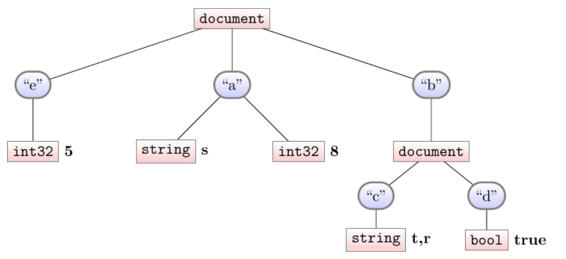
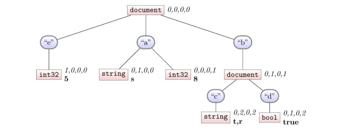
Design: The schema illustrations above are quite close to our in-memory representation. Our schema is a tree: the blue nodes represent the names, mapping closely to the typical b.c way of referring to a field in a (nested) document. The square nodes maintain what types we’ve seen under that key-path.
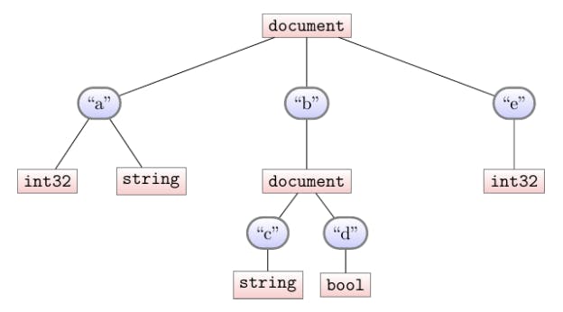
The schema of multiple documents is naturally defined by the union (or merge) of each document’s individual schema. So the schema for our four-document collection is:
A few highlights:
-
Note that we don’t preserve the “frequency” of keys. Our schema doesn’t distinguish whether a field appears in every document, or just some documents.
-
Merging schemas is commutative; we’ll always get the same schema no matter the order we visit the documents.
The schema information is enough for us to tell the parquet file what columns it will need, so we can start laying it out. Roughly, each leaf (representing a scalar value in our schema, such a string or integer) will map to a column in the parquet file. Typically we’d name each column based on the names we see on the path from the root to that leaf. For instance, in this tree we’d have b.c and b.d as two column names. The atypical case is in supporting polymorphism. See how in our example the name a refers to two different parquet columns: one of type int32, and another as type string. In these cases we disambiguate the columns by appending their type-name at the end. So the 5 columns from this schema will be named: a.int32, a.string, b.c, b.d, e.2
Code to build the schema
We know we need our schema, and we know what it should look like. All that’s left is writing code to actually compute the schema. We can compute it inductively:
-
Start with an empty schema
-
On the next document, walk that document’s tree-structure and the schema-tree in lockstep. If there is ever a node in our document that is missing from our schema-tree, add that node.
-
Repeat step-2 for the next document until done.
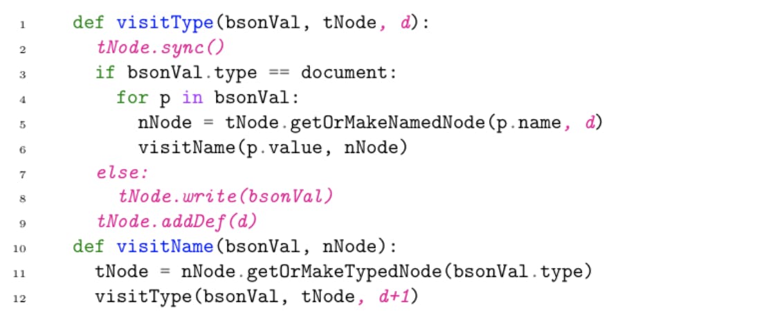
At the end of each step-2, the schema we have built is the schema for all the documents-seen-so-far. Here is some pseudocode describing step-2 in more depth:
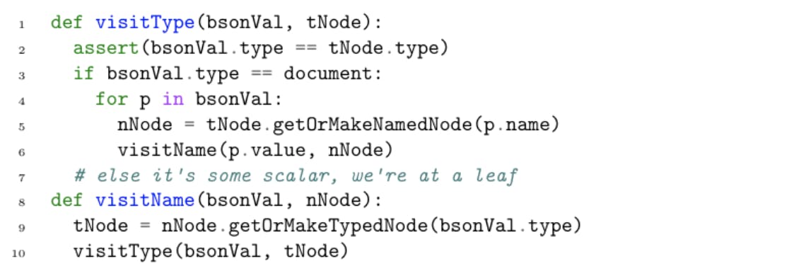
The first parameter of each function is the document we’re walking, and the second parameter is the current schema-tree-node we’re in. The visitType function refers to the square nodes in our tree, and the visitName function to the round nodes. Note how on line 6 we are recursing into the individual key-value pairs of our document: that’s our actual tree-walk.
To illustrate its implementation, here is how we’d iteratively build the schema over our four documents. Each image is the schema after step-2. We yellow-highlight the nodes to indicate those nodes we allocate, or visit, as we traversed the latest document.
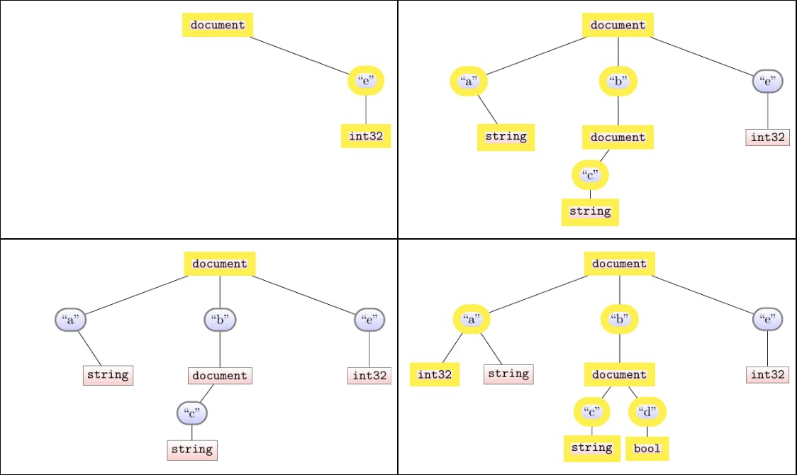
Note that this walk is driven by the document-size: even if our schema is ultimately very big, the time it takes to process a document is only dependent on the size of that document. When we shred document 3, we only visit the root, for instance.
Hooray! This document-driven approach was our first step towards performance improvements in parquet-writing. Previously we had a more schema-driven approach that used more allocations and node-traversals. We’re ready to extend this foundation and shred our documents in the same pass. Before we jump in, let’s conclude with one crucial invariant that is apparent as a result of how we build our schema:
Online schema invariant
Once we place a leaf node in our tree, the path to that leaf never changes. In other words, we only ever place new leaves; we never insert a node “above” an existing one. We will rely on this invariant heavily to show that we’re correctly maintaining the structural metadata in the course of shredding.
Introducing shredding
We can now rest assured that, when the time comes to create a parquet file, we will have the right schema-information to tell it what columns to create. Of course, now we need to get the actual data to fill in those columns.
Recall one of the key challenges we anticipated was maintaining the metadata. This metadata is what parquet needs to remember the structure of each document. These are called definition levels and repetition levels. Each column in parquet, in addition to its data-actual column, can have two more columns of this additional metadata. 3 Before exploring how our shredding builds and maintains this information, let’s take a brief detour to build an intuition about how this metadata works.
Using definition and repetition levels
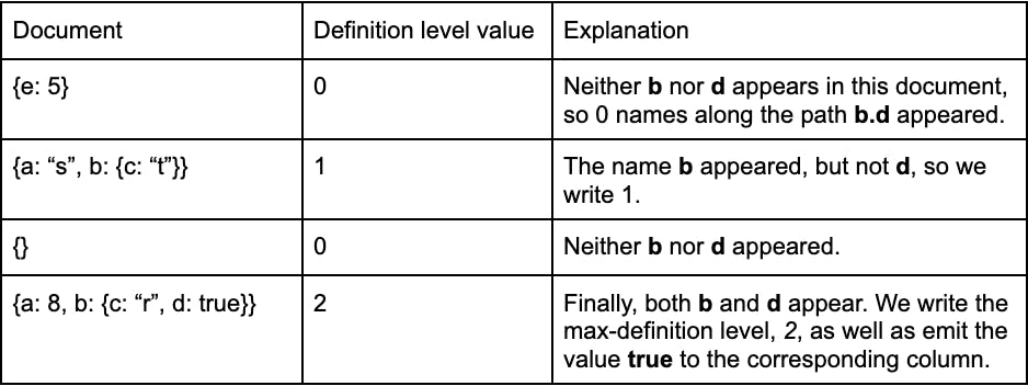
Say we’ve naively shredded our 4-document stream without regard to any metadata. For visualization, we’ll attach the column-contents to each leaf in our schema. So after shredding our data looks like:
This presents a challenge. Say one day we want to re-assemble our documents. What would our documents look like? We might very well guess the correct sequence, but absent additional metadata, we might as well reassemble this data into something like:
-
{a: 5, b: {c: “s”, d: true}, e: 8}
-
{a: r, b: {“t”}}
Plainly these are very different from our original documents. That’s not good! So we need a way to disambiguate our shredded values; repetition and definition levels enable this in parquet. The full explanation can be found in the Dremel paper4 (see also this very clear 2013 Twitter blog post5). For brevity, here we’re just going to be looking at definition levels. Repetition levels are different of course, but similar enough where the mechanisms we’ll ultimately highlight will work the same way. We elide discussing repetition levels for brevity.
Definition Levels: The i-th definition level in a column indicates how many names along the path to that column were present for document i6. This means as we process a document, we promise to write some definition-level for each leaf7. To introduce this idea, consider the leaf b.d. After processing all documents, it will have the definition levels "0,1,0,2". Here is how these b.d definition-levels are derived as we process our four documents.
Now we can consider how our whole tree looks with all the definition levels.
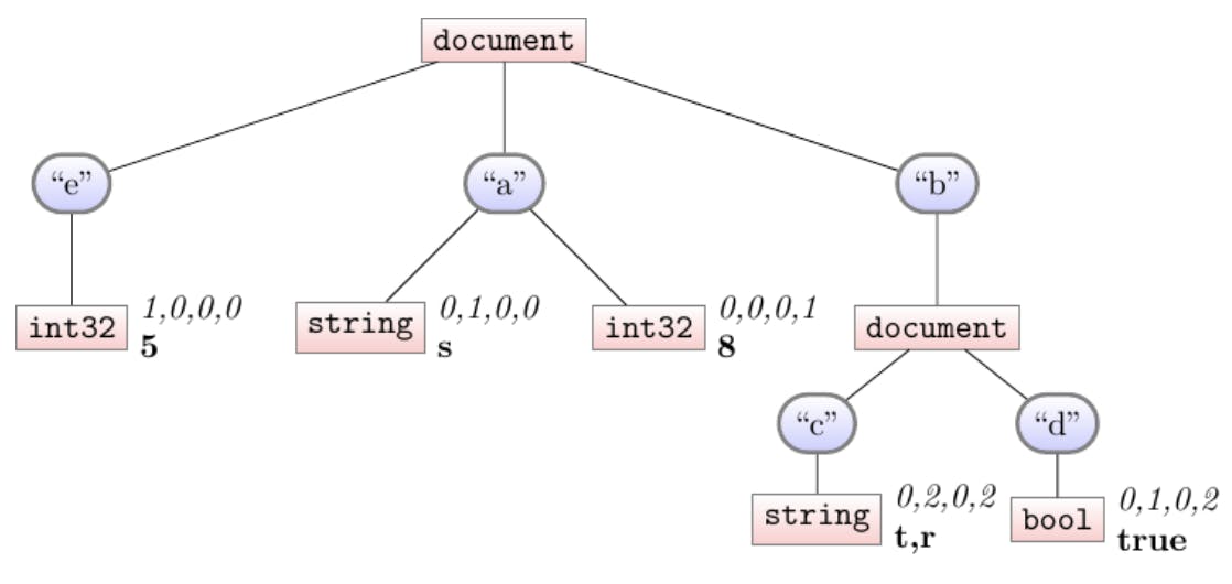
This picture tries to demonstrate a lot of the impact of definition-levels. Some highlights:
-
Consider column e: It has definition levels 1, 0, 0, and 0. The 1 indicates that the first document ({e:5}) has 1 name defined along the path to e. Said another way, that first 1 indicates that the value in the column-store, 5, is present in the first document. As e does not appear in any other documents, it has 0 for the rest of its definition-levels.
-
We discussed column b.d, with def-levels 0, 1, 0, 2 above. We can compare it to its sibling, b.c. In particular, this highlights how the number of values a column has is exactly equal to the number of times the max-definition-level appears. The definition-level stream for b.d only has the max-definition-level, 2, once. It only has one value: true. Its sibling, however, has the max-definition-level, 2, twice, and correspondingly has two values.
-
Columns a.string and a.int32 show that even though the name a appears in two document streams, we have to disambiguate the underlying data-type. This is saying that the second document contains a as a string, and the fourth document contains a as an int32. This is a detail that reveals some of the extra work we take to translate polymorphic documents into parquet-amenable formats.
Hopefully this suggests a reassembly-into-documents algorithm: for the i-th document, we look at the i-th def-level of each column. When it’s equal to the number-of-names on our path, we pop off the next value in the value-stream associated with that column. There are more complications and subtleties in practice, but this captures the spirit of it.
Code to shred the document stream
We’ve covered how definition levels are used to reassemble the original documents. Now we can turn to our task of actually computing the definition levels as we shred our documents. Two challenges present themselves:
-
We want to emit the correct definition-level as we process each document, but that definition level implicitly depends on the structure of the schema (it’s “how many names were on that path”). We’re building our schema on-line—how can we be confident that the definition level we write shouldn’t have been different as the schema grows to accommodate more documents?
-
If the 10th document introduces some column named z, then we clearly haven’t been adding any definition levels to that column for the past 9 documents—we didn’t know the column existed yet! How might we “backfill” the required def-levels? It’s not enough to simply fill them with 0s, because (recall our 2nd example document, the b.d path) sometimes we need an intermediate def-value.
The first challenge is easily addressed: recall the crucial Online Schema Invariant, that a path to a leaf never changes. A consequence of that invariant is that we can be confident in the definition-levels for any leaf. Its depth (i.e., the number of names to that leaf) is not going to change. Hooray! Hopefully as-presented this punchline is very clear and obvious to you; during the course of development, however, this result took some careful reasoning to establish.
It is the second challenge that requires even more thought. Ultimately we found we could leverage the “lazy syncing” of def-levels the Dremel paper introduces.8 We were already interested in using it to keep our per-document walk proportional to the document size, but it was a happy moment to see it could help us in the new-column case. Lazy syncing is mechanically simple but conceptually subtle, let’s dive in.
Lazy syncing
To set the stage for lazy syncing, we extend our definition-streams to interior (type-)nodes. In our example, that means our final shredding would look more like:
See how the two document nodes now have definition-levels. The definition levels express the same idea: how many names did we see along this path for the i-th document. Let’s walk through our four-document example one more time, now shredding in addition to building the schema.
Shredding document 1
This is the simple case. This is our first-ever document, so we know there’s no def-levels to “backfill”, and no nodes we’re trying to skip. We highlight the nodes where we’re adding definition-levels.
Shredding document 2
Now things are getting interesting. We don’t highlight the e column because our algorithm doesn’t touch it for document 2. We do, however, inevitably touch one of its ancestors (in this case, the root).
Syncing: When we create the a, b, c columns, how did we know to backfill the definition levels for the first document all with 0? This is because as we write the def-level of the current document, we first always check to make sure we’re in sync with our parent for any prior documents, and so on transitively. To narrate an example of syncing: When we created the a column, our code basically said “and your second document def-level is 1”. You might imagine the a column panicking–it never heard what its first document def-level is! What might you do when you panic? You might talk to your parent: in this case a’s parent is the root, and a asks “what did you see for the first document?” — the root says 0, and a can trust that 0 is the deepest the first document ever got to a.
For a more complicated case, see what happens with b and b.c. In that case, they both were written-to for the first time in this document. They were both initially skipped, so they both learn 0 from their parent (transitively), but of course b.c was written-to in this document, so it stops syncing at that latest document and writes a 2 instead of the 1 that b writes.
We only sync a column when we write to it. In particular, see how we don’t sync the def-levels for e. This subtlety is key to enabling us to shred documents efficiently: when we shred a document, we only have to traverse the nodes in that document, not the (potentially much larger) number of nodes in the whole schema.
This is syncing in-action. Let’s see a few more examples.
Shredding document 3
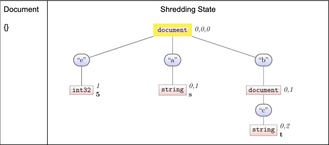
This is a sort-of easy case: we hardly write anything. Instead of (for now) having to walk the whole schema, we’re only touching the root node—after all, we don’t have much more information to write for the empty-document. Implicitly, we’re relying on the syncing machinery to ultimately propagate this information as required.
Shredding document 4
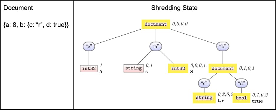
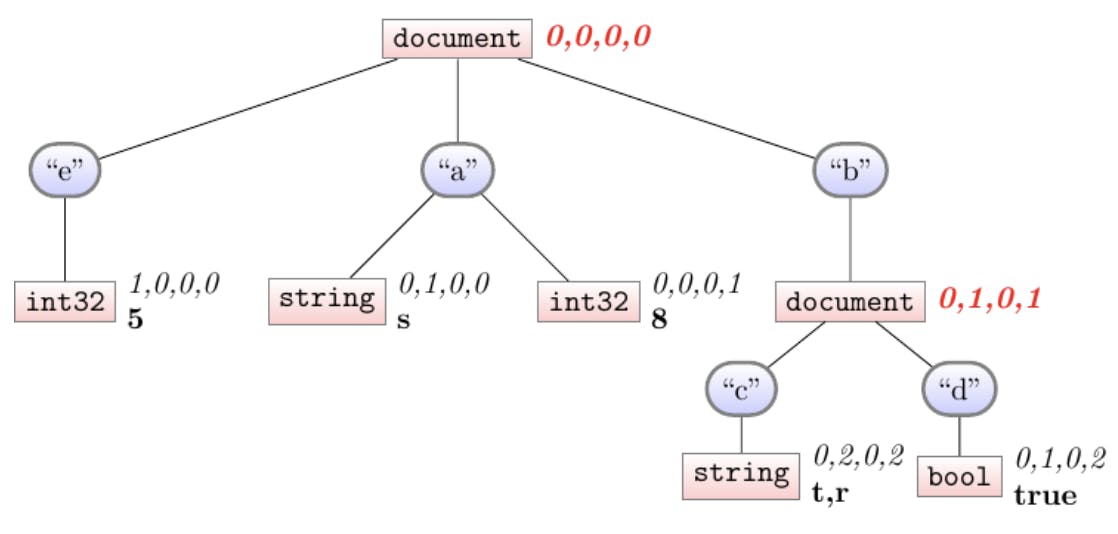
We finally ingest our last document. See in particular how the new-to-us column of b.d is able to sync the previous 3 def-levels from its parent, correctly learning the “1” for the second row. Almost without noticing, our syncing machinery gives us the ability to handle entirely-new columns: we simply create the new column, and then sync with its existing parent. The only thing we need to rely on is that we have some global ancestor that sees every document: but of course, that’s exactly the root, as we saw with Document 3.
Finally, note also that this doesn’t quite look like the final form we expected: we ultimately do need 4 def-levels on every leaf. One last “global-sync”, where we propagate the defs down to the leaves until everyone’s caught up, finalizes our shredder-state into what we expect:
Phew, the pseudocode
Congratulations on getting through all that shredding. Hopefully this has been a thorough illustration of how this one key technology, syncing, enables us to extend our shredder to handle new columns as they appear online. While conceptually nontrivial, the (pseudo)-code extends easily from our schema-building example. To drive that home, the code-diffs are highlighted in magenta. It’s not that big of a diff to get full shredding!
Concluding the implementation
We are now able to take a stream of documents and shred those documents into an in-memory columnar format complete with their structural metadata. We only ever need to look at each document once for this process, leading to a substantive performance improvement. What we have not explored, and won’t in this blog post, are all the extra details we need to get this functional: swapping our in-memory representation to disk as-needed to bound our memory usage, actually emitting our in-memory representation into the physical Parquet file (thanks to the apache-go library), and more.
Getting the new approach in production
While the shredder algorithm is a fascinating component, it is just one part of the larger process of delivering product improvements. Any large deliverable involves many people, and anything that impacts our users calls for meaningful validation. We’ll conclude our discussion of shredding by placing its work and impact in this larger context.
Build together
This work benefited greatly from a number of collaborators. We were fortunate to be able to draw on a diverse range of experts and collaborators for this work, and doubly-so because so many of us were able to learn from each other along the way.
-
A distinguished engineer pushed for this project, drawing her analytics expertise to show how we could have a much more column-first perspective on parquet emission, ultimately leading us to adopt the official apache arrow project as our parquet-file-writing library, interfaced with via the above-described shredder. She also outlined a lot of the key requirements for our swap-to-disk procedures, in addition to teaching me and other colleagues an enormous amount about the analytics world.
-
At the cross-team level, we sought out performance-measurement experts to help characterize what performance success should look like at a systems level.
-
At the individual collaboration level, I was glad for the privilege of introducing several junior colleagues to performance work and how to get effective measurements. Their contributions included many other technical deliverables that substantially improved our product’s performance, and insightful ways of measuring performance.
Validating the behavior
Finally, for all the technical and collaborative work we’ve discussed, the value of the work is predicated on us getting this into production. The popularity and importance of our parquet-writing motivated this work and made us excited to release it as soon as possible. By the same token, we needed to release this without compromising stability or correctness. That’s part of being a developer data platform.
Along with table-stakes validation like targeted unit-tests validating the core machinery, integration tests validating how that machinery is used by the larger product, and end-to-end tests validating the, well, end-to-end experience, we sought out synthetic and real-world datasets to make sure we handled input of all shapes and sizes. We also strived to validate our project from a customer’s perspective: people emit parquet files with the intention of using them elsewhere, so we extensively tested our produced parquet files with third-party readers to assure their compatibility.
Ultimately, the performance improvement brought on by this work is considerable. For our largest customers, our logging metrics indicate we’ve over doubled our parquet-writing throughput. This is consistent with our customer-oriented internal benchmarks, and the effect is that we are now saving many compute-days per day servicing our customer requests. We believe this work has laid a strong foundation for our parquet-emission support.
Thanks for reading!
1 For those familiar with the parquet-specific term, we are able to flush on each rowgroup, not just the whole file–but the issue and challenge remains the same. We write “file” here for simplicity.
2 Note that a typename, such as “.int32” or “.string”, will only appear at the end of a path.
3 Not all columns require these streams, here we’re referring to the general case. For more details, see the Dremel paper, cited below.
4 https://dl.acm.org/doi/abs/10.14778/1920841.1920886
5 https://blog.twitter.com/engineering/en_us/a/2013/dremel-made-simple-with-parquet
6 For those already familiar with parquet: technically the definition level range is only for names-that-could-possibly-be-missing, i.e., excluding fields marked REQUIRED. For our discussion and simplicity, we’re assuming all columns are OPTIONAL.
7 Things get a little more complicated when also considering repetition levels (multiple definition levels might map to one document), but again for brevity we do not discuss repetition levels.
8 Section 4.2, and Appendix A, of the Dremel paper.